11  Doctors across the world: making maps with ggplot2

In this chapter we’ll learn how to identify open data sources, make maps with ggplot2 using data from the maps package, and create title panels with an unorthodox use of facets.

Packages required in this chapter:

library(dplyr)
library(ggplot2)
library(ggtext)
library(MetBrewer)
library(readr)
library(showtext)
library(sysfonts)

11.1 Data

We’ll visualize data on Medical doctors per 1,000 people using the dataset from the Our World in Data website (ourworldindata.org) (Our World in Data 2019). The aim of Our World in Data, according to their website, is to publish the research and data to make progress against the world’s largest problems. There are datasets on everything from energy and environment, to poverty and education, to name a few. Their website also has many examples of beautiful, effective data visualizations if you’re ever looking for inspiration.

You can either download the CSV file from ourworldindata.org/grapher/physicians-per-1000-people manually or you can do as we did in Chapter 6, and download it directly into R using the URL. Simply pass the URL into the read_csv() function from **readr``** (orread.csv()` from base R if you prefer). As in Chapter 6, we split the URL into the base URL and the specific page of interest to make it easier to later load in other datasets if we choose to.

base_url <- "https://ourworldindata.org/grapher/"
url <- paste0(
  base_url,
  "physicians-per-1000-people.csv"
)
doctors <- read_csv(url)

Tip 11.1: Connecting to Our World in Data via R

The owidapi R package (Scheuch 2025) provides an R interface to the Our World in Data website, allowing you to search and download data in R without having to navigate through the website. However, it’s not much less complicated than passing in the URL to read_csv().

library(owidapi)
doctors <- owid_get("physicians-per-1000-people")

Previously the owidR package (York 2023) also provided a similar interface, but at the time of writing, it hasn’t been updated to use the newest Our World in Data API which results in errors when accessing data.

Tip 11.2: Saving data for later use

You may choose to save a copy of doctors as a CSV file for later use by using write.csv() or write_csv() from readr``**. This means you don't have to download the data each time you open R and don't have to worry about the data updating when you're halfway through your analysis. You can then later read in the data withread.csvorread_csv()from **readr``.

Tip 11.3: Finding sources of data

There’s often a Bring Your Own Data week each year of TidyTuesday (R4DS Online Learning Community 2023), where participants are encouraged to source their own data. Some use their own data - visualizing how many times they’ve gone for a run over the past year, or recreating GitHub contributions graphs. Others choose to find and visualize other sources of data. So where do you find publicly available data?

There are many open sources of data, covering a wide range of topics, time frames, and regions across the world. Some government organisations have data portals, some companies have APIs you can access, some academic papers have accompanying data, or the Google dataset search engine (datasetsearch.research.google.com) might also help you to identify data you’re interested in.

11.2 Exploratory work

Let’s start by exploring the data to see if there are interesting patterns that can be visualized.

11.2.1 Data exploration

The data is reasonably small, containing only 4 columns: Entity (denoting the country or a larger region), Code (the country code), Year (year the data relates to), and Physicians (per 1,000 people). The 4939 rows of data cover 222 different regions (some aggregates of others), with data covering 62 years.

head(doctors)

# A tibble: 6 × 4
  Entity      Code   Year `Physicians (per 1,000 people)`
  <chr>       <chr> <dbl>                           <dbl>
1 Afghanistan AFG    1960                           0.035
2 Afghanistan AFG    1965                           0.063
3 Afghanistan AFG    1970                           0.065
4 Afghanistan AFG    1981                           0.077
5 Afghanistan AFG    1986                           0.183
6 Afghanistan AFG    1987                           0.179

Often when there’s a time component to data, one of the most obvious patterns to consider is how other variables change over time. Although line charts are probably most common for visualizing time series data, a simple scatter plot can also indicate if there’s a general trend in the data. Sometimes scatter plots also look cleaner than line charts - a line for each region in this chart would very much look like a spaghetti chart as discussed in Chapter 3.

plot(
  x = doctors$Year,
  y = doctors$`Physicians (per 1,000 people)`,
  xlab = "Year",
  ylab = "Physicians per 1,000 people"
)

Figure 11.1: Simple non-styled scatterplot of number of physicians per 1,000 people over time showing an increasing trend, created in base R.

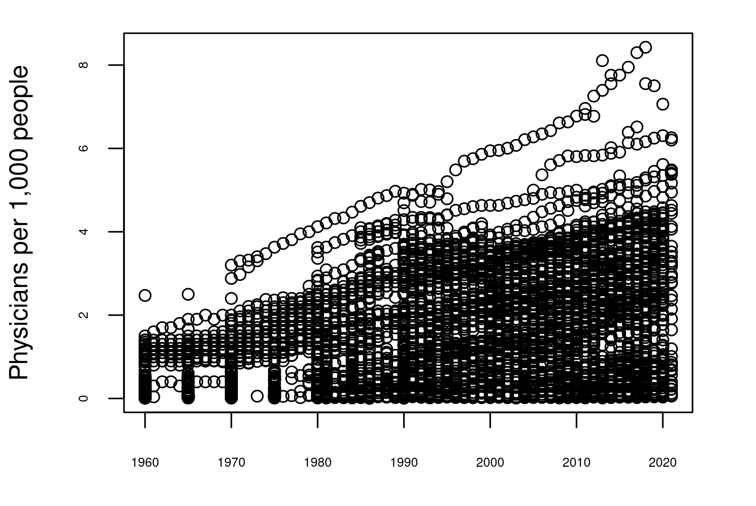
There seems to be a general increasing trend between 1960 and 2020. The other important component of this data that we may want to explore is the spatial aspect - is there a pattern over space as well as over time?

11.2.2 Exploratory sketches

The most common approach to visualizing spatial data is, of course, to plot it on a map. If the aim is to show how a variable changes across different countries (or other defined regions), it’s very common to color the country based on the value of the variable. These are often termed choropleth maps.

Figure 11.2: Initial sketch of a map of the world, showing title enclosed in a box and legend positioned horizontally in the bottom right

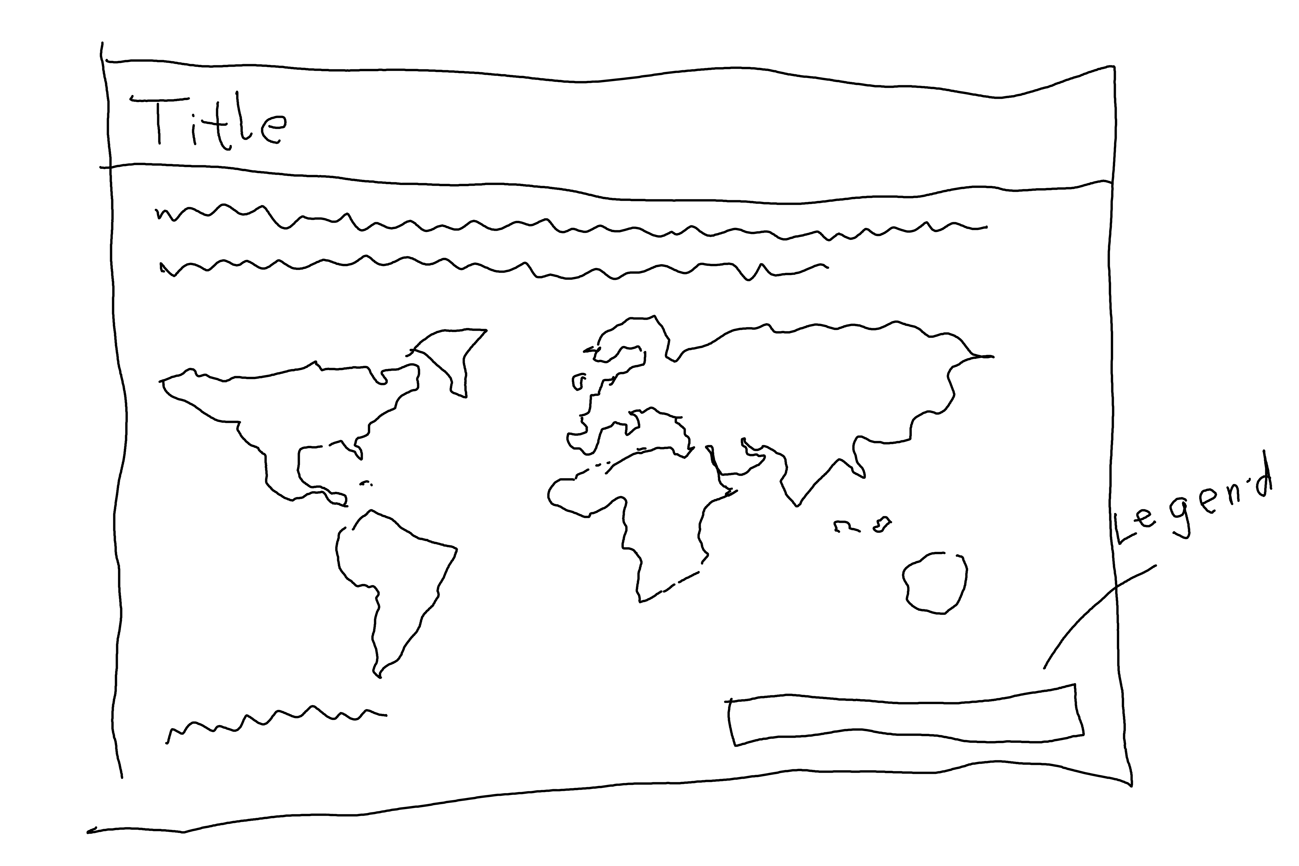
At this point, it’s also often a good time to start thinking about the orientation and aspect ratio of the plot you’ll create. This will depend a lot of where the plot is going to end up - for example, plots in a single column academic article will typically be landscape graphs. The choice of orientation and aspect ratio can also affect how clearly your data is displayed - choosing a very wide plot for time series data can stretch the series and obliterate any appearance of trend. With maps, you’re a little bit more constrained because there is already an underlying aspect ratio in the plot you’re creating. For this map, a landscape orientation with a 6x4 aspect ratio should work reasonably well.

11.3 Preparing a plot

To create the map sketched out in Figure 11.2, we need to do two things (i) decide which data to plot: which regions, and which years; and (ii) source some spatial data beyond just region names and country codes.

11.3.1 Data wrangling

Since this data is already fairly tidy, there isn’t too much data wrangling to be done. The only processing we really need to do is getting rid of the data we don’t need, and renaming a couple of columns to make them easier to work with. We can use the rename() function from dplyr to rename the Entity column to region (for reasons that will become clear in the next paragraph!). We also rename the Physicians (per 1,000 people) column to doctors to make it easier to work with, and rename Year to year for consistency. The data has multiple entries for each country, spanning different years. We could make an animated map to show how the number of doctors is changing over time, but for now we’ll keep it simple with a static map showing a snapshot at one point in time. However, there’s a bit of a problem. If you inspect the data, you’ll see that not every country has an entry for each year - let’s use the most recent data available for each country. For each region, we keep the row with only the most recent year using a combination of group_by() and slice_max() from {dplyr}.

doctors <- doctors |>
  rename(
    year = Year,
    region = Entity,
    doctors = `Physicians (per 1,000 people)`
  ) |>
  select(region, year, doctors) |>
  group_by(region) |>
  slice_max(year) |>
  ungroup()

To plot this data on a world map, we also need data for the country borders. Luckily, the map_data() function built into ggplot2 can help us with that! This function takes data from the maps package and turns it into an object you can plot directly with ggplot2.

world <- map_data("world")

Of course, it’s never quite that straightforward. We need to join the world map data to our doctors data, and to do that we need a column in each data sets to join by - we’ll use the region column. If you try to join these two data sets using the region column, you’ll notice that you end up with some unexpected NA values. So what’s going on?

Tip 11.4: Renaming columns

You don’t need to rename columns in your data to be able to join them, but you may find it easier to work with the data after renaming Entity to region to maintain consistency across datasets.

There are two issues here. Firstly, there are more regions in the world data than there are in the doctors data:

length(unique(world$region))

[1] 252

length(unique(doctors$region))

[1] 222

This is partly due to the fact that the doctors data has implicitly missing values - if no data is available for a region, no rows exists in the data for that region. It isn’t listed with NA values. Note that there are also some regions in doctors which do not exist in world - for example, the entity "Upper-middle-income countries" is listed within doctors.

Secondly, if you inspect the region names, you’ll see that for some countries, their names are encoded differently. For example, in the world data, the United States is listed as "USA" whilst in the doctors data, it’s listed as "United States". Here, the easiest thing to do is manually rename the values that differ in one of the datasets. We can use the recode() function from dplyr to do that. Note that recode() has the rather unusual (for the tidyverse) syntax of old_name = new_name:

plot_data <- doctors |>
  mutate(
    region =
      recode(region,
        "United Kingdom" = "UK",
        "United States" = "USA",
        "Democratic Republic of Congo" = "Democratic Republic of the Congo",
        "Cote d'Ivoire" = "Ivory Coast",
        "Congo" = "Republic of Congo",
        "Czechia" = "Czech Republic"
      )
  )

The entries in the region column of doctors that don’t correspond to countries e.g. "Upper-middle-income countries" are not values that are required for the map. Therefore a left_join() can be performed, with world on the left - keeping all the countries listed in world and joining only those with a corresponding value in doctors. The remaining countries in world with no match in doctors are listed with NA values. The rows for "Antarctica" are filtered out - Antarctica is often given a disproportionate amount of space on world maps (at least those not centered on Antarctica) in the process of projecting a sphere onto a rectangle.

map_data <- left_join(
  world,
  plot_data,
  by = "region"
) |>
  filter(region != "Antarctica")

Now, we have everything we need to create a simple map.

11.3.2 The first plot

We start, as almost always, with the ggplot() function, and pass in the data and aesthetic mappings that will apply to the whole plot. The longitude (long) and latitude (lat) are passed to the x and y axes; and we specify that the fill color of each country should be based on the doctors column. We also specify map_id - an aesthetic mapping that isn’t seen as often as the others. This is used to tell geom_map() which column defines each region polygon (not entirely unlike the group aesthetic). Then, we use geom_map() to actually draw the map.

Tip 11.5: Alternatives to geom_map()

Both geom_sf() and geom_polygon() can be used as an alternative to geom_map() for creating maps within ggplot2.

However, they expect different formats of data. The geom_sf() function expects an sf object, in contrast to geom_map() which works with coordinates as columns in a data.frame or tibble. For examples of using geom_sf(), see Chapter 12.

You could also use geom_polygon() to plot map_data instead of geom_map(), but it makes it more difficult to project the map in the way we want to.

basic_plot <- ggplot(
  data = map_data,
  mapping = aes(
    x = long,
    y = lat,
    map_id = region,
    fill = doctors
  )
) +
  geom_map(map = map_data)
basic_plot

Figure 11.3: Map of the world with countries colored based on number of doctors per 1,000 people. The map looks stretched.

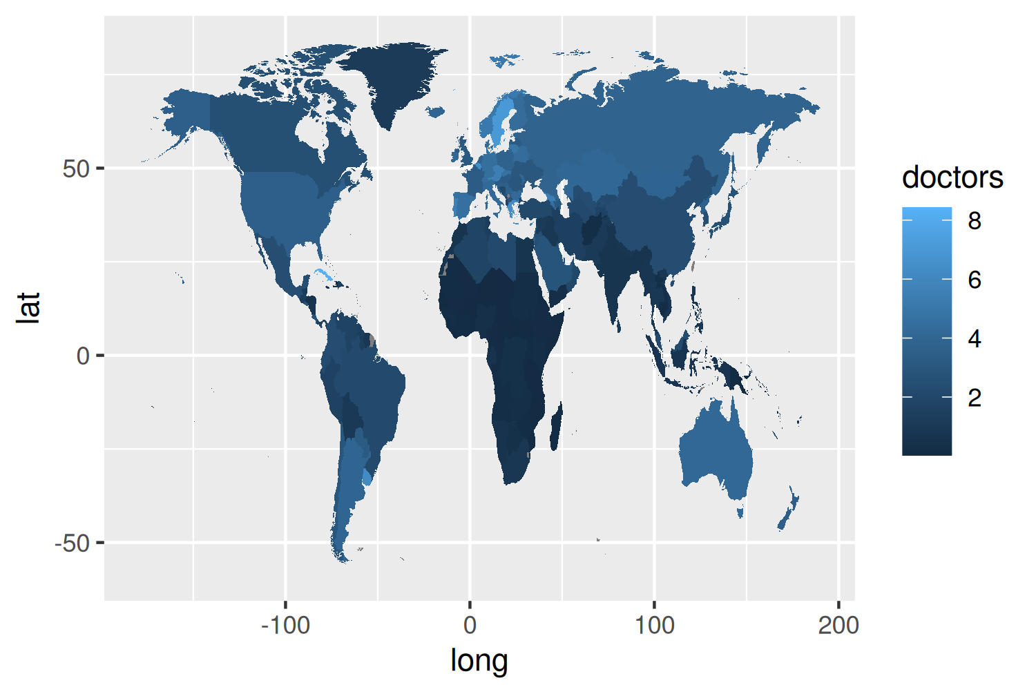
We now have a simple map that shows our data, but there are several problems with it:

• The map looks as if someone has stretched it vertically, since there’s no map projection specified. Countries are still recognizable, but not quite the right shape.
• The color palette is not ideal. It’s more intuitive for brighter or lighter colors to represent smaller values, and for darker colors to represent higher values - at least for light colored backgrounds (Schloss et al. 2019). The default gradient color scale in ggplot2 is the opposite way around.
• There are labels that don’t need to be there (lat and long), and missing labels that should be there (title and subtitle, for example).

So let’s fix those elements of the initial plot.

11.4 Advanced styling

We’ll start by considering alternative color palettes, then think about what text that should be added, before finalizing the layout.

11.4.1 Colors

There are many, many color palette R packages in existence, and even more outside of the R ecosystem. In fact, the paletteer package (Hvitfeldt 2021) is designed to give a common interface to a comprehensive collection of color palettes in R. A popular color palette R package is MetBrewer (Mills 2022) - a collection of color palettes inspired by works of art at the Metropolitan Museum of Art in New York. It has many beautiful palettes, and many that work in traditional data visualizations. You can view all available palettes using display_all(colorblind_only = TRUE). Since doctors is a continuous variable, we’ll look at the sequential palettes only.

MetBrewer does have functions that interface directly with ggplot2 (such as scale_fill_met_c()) but we’re going to use some of the colors in the palette to also define variables for the highlight and text colors. To get a good range of colors, we extract 20 colors from the "Hokusai2" palette. The text_col is the 18th color and highlight_col is the 15th color. A variable containing the background color, bg_col, is also defined.

library(MetBrewer)
col_palette <- met.brewer("Hokusai2", n = 20)
text_col <- col_palette[18]
highlight_col <- col_palette[15]
bg_col <- "#EADEDA"

These colors can then be passed into scale_fill_gradientn() from ggplot2. The limits of the color scale can also be set. Rather than adding labels for values on the legend, we can add text labels for Fewer doctors and More doctors. These are positioned 0.8 in from the limits of the color scale.

col_plot <- basic_plot +
  scale_fill_gradientn(
    colors = col_palette,
    limits = c(0, 10),
    breaks = c(0.8, 9.2),
    labels = c("Fewer doctors", "More doctors")
  )
col_plot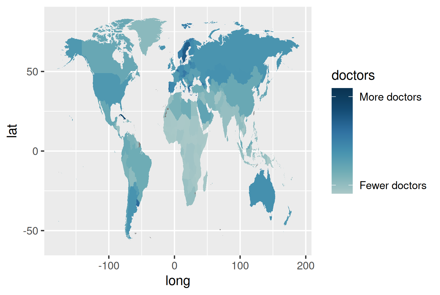

Figure 11.4: Map of the world with countries colored based on number of doctors per 1,000 people, showing a different color scheme.

11.4.2 Text and fonts

As in previous chapters, fonts can be defined using the sysfonts and showtext packages. Here, the Roboto typeface is loaded through Google Fonts for the main font used, and Roboto Slab is loaded for use in the title.

font_add_google(name = "Roboto")
font_add_google(name = "Roboto Slab")
showtext_auto()
showtext_opts(dpi = 300)
body_font <- "Roboto"
title_font <- "Roboto Slab"

Now, we can define some text for the title, subtitle, and caption. As in previous chapters, we’ll be using ggtext for formatting which means we can use HTML syntax to add line breaks.

title <- "Doctors across the world"
subtitle <- "This map show the number of doctors per thousand people, revealing which countries* may be more likely to struggle in providing care for a population.<br><br>*using the most recent available data for each country."

Let’s create a custom caption that includes Font Awesome icons, as described in Chapter 7, which is passed into the source_caption() function we defined in Chapter 6:

social <- social_caption(
  icon_color = highlight_col,
  font_color = text_col,
  font_family = body_font
)
caption <- source_caption(
  source = "Our World in Data",
  sep = "<br>",
  graphic = social
)

These text variables can then be passed into the labs() function.

text_plot <- col_plot +
  labs(
    title = title,
    subtitle = subtitle,
    caption = caption
  )

To apply our chosen typefaces to the plot, the theme elements need to be adjusted.

11.4.3 Adjusting themes

We start by adding theme_void() from ggplot2. The theme_void function removes all theme elements - including grid lines, axis labels, and the background. The legend and specified titles and subtitles remain. This theme is especially useful for maps where it’s more common for axis lines, axis titles, and grid lines not to be displayed. Like other built-in theme options, we can still set the base_size and base_family to set the default size and typeface for any text that is displayed.

We also set the plot.title, plot.subtitle, and plot.caption to use element_textbox_simple from ggtext to allow the markdown syntax and automatically wrap long subtitles as we’ve seen in previous chapters.

text_plot +
  theme_void(base_size = 8, base_family = body_font) +
  theme(
    plot.margin = margin(10, 10, 10, 10),
    plot.background = element_rect(
      fill = bg_col, color = bg_col
    ),
    panel.background = element_rect(
      fill = bg_col, color = bg_col
    ),
    plot.title = element_textbox_simple(
      color = text_col,
      family = title_font
    ),
    plot.subtitle = element_textbox_simple(
      color = text_col
    ),
    plot.caption = element_textbox_simple(
      hjust = 0,
      color = text_col
    )
  )

Figure 11.5: Map of the world with countries colored based on number of doctors per 1,000 people. The map looks stretched, and the fonts in the title and subtitle are close together.

One of the aesthetic design choices we might want to make here, is to include the title within a banner with a different colored background. Although this might seem like a fairly straightforward thing to want, it’s actually not that easy with ggplot2. There are some solutions to the problem using packages like cowplot (C. O. Wilke 2024) or grid (R Core Team 2024) to draw rectangles and text. But we can do this within ggplot2 - by using facets in a way they were not designed to be used. Let’s start by adding an additional column called label to map_data that contains the title (for every row in the data):

map_data$label <- title

Tip 11.6: Choosing a column name

This column does not need to be called label, you can use any name you choose as long as it’s not an existing column.

You could also pass the title directly into facet_wrap() instead of creating a new column:

facet_wrap(~"Doctors across the world")

Then we can use facet_wrap() and facet across the label column. Since there’s only one value of label in the data, this just adds the title as strip text at the top of the plot. While we’re here, let’s make the country outlines in the map the same color as the background, and make the lines a little bit thicker.

styled_plot <- ggplot(
  data = map_data,
  mapping = aes(
    long,
    lat,
    map_id = region,
    fill = doctors
  )
) +
  geom_map(
    map = map_data,
    color = bg_col,
    linewidth = 0.3
  ) +
  scale_fill_gradientn(
    colors = col_palette,
    limits = c(0, 10),
    breaks = c(0.8, 9.2),
    labels = c("Fewer doctors", "More doctors")
  ) +
  labs(
    title = title,
    subtitle = subtitle,
    caption = caption
  ) +
  facet_wrap(~label) +
  theme_void(base_size = 7, base_family = body_font) +
  theme(
    plot.margin = margin(10, 10, 10, 10),
    plot.background = element_rect(
      fill = bg_col, color = bg_col
    ),
    panel.background = element_rect(
      fill = bg_col, color = bg_col
    ),
    plot.title = element_textbox_simple(
      color = text_col,
      family = title_font,
      lineheight = 0.5
    ),
    plot.subtitle = element_textbox_simple(
      color = text_col,
      lineheight = 0.5
    ),
    plot.caption = element_textbox_simple(
      hjust = 0,
      color = text_col,
      lineheight = 0.5
    ),
    strip.background = element_rect(
      fill = highlight_col, color = highlight_col
    )
  )
styled_plot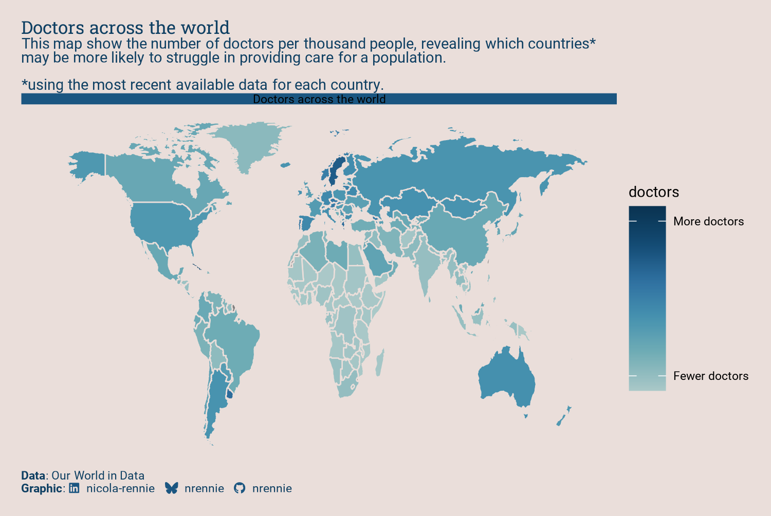

Figure 11.6: Map of the world with duplicated title in the facet strip text, with dark text against a dark blue background.

It’s obvious that there are some issues with this plot now that the strip text contains the title:

• There is a duplicate title set using labs(), and the strip.text title is too dark to read against the blue background.
• The subtitle is above the title.
• The map still appears stretched.
• The legend is taking up quite a lot of space, and the white ticks in the colorbar are distracting.

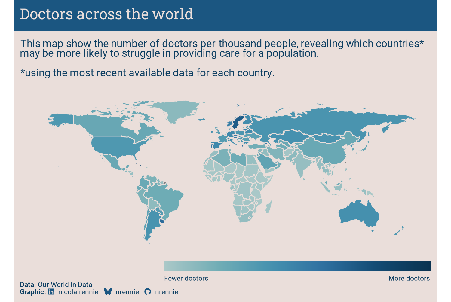
To solve the first two problems, the title and subtitle arguments of labs() can be set to NULL to remove them from the plot. Instead, the tag argument in labs() can be used to set the subtitle. The nice thing about using tag is the plot.tag.position argument within theme() which allows you to position the text anywhere on the plot. The strip.text and plot.tag arguments of theme should also be set using element_textbox_simple() from ggtext to allow the text to be styled as we wish. The top, left, and right margins of the plot should be set to 0 using plot.margin to make sure that the strip text banner goes to the edge of the plot.

To solve the third problem of the map looking stretched, we can apply coord_sf() which applies the World Geodetic System 1984 (WGS84) CRS (coordinate reference system). Chapter 12 discusses coordinate reference systems in more detail. The upper limit of the y axis can also be extended beyond the range of the data to make room for the subtitle added using tag.

styled_plot2 <- styled_plot +
  labs(
    title = NULL, subtitle = NULL, tag = subtitle
  ) +
  # add space for the tag (subtitle) text
  coord_sf(ylim = c(-60, 140)) +
  theme(
    # move and format the tag (subtitle) text
    plot.margin = margin(0, 0, 5, 0),
    plot.tag.position = c(0.015, 0.8),
    plot.tag = element_textbox_simple(
      color = text_col,
      lineheight = 0.6,
      hjust = 0,
      maxwidth = 0.98
    ),
    # add margin for caption
    plot.caption = element_textbox_simple(
      hjust = 0,
      color = text_col,
      margin = margin(l = 5),
      lineheight = 0.6
    ),
    # change title text color
    strip.text = element_textbox_simple(
      color = bg_col,
      family = title_font,
      margin = margin(7, 5, 7, 5),
      lineheight = 0.6,
      size = rel(1.7)
    )
  )

Note that the values used in plot.tag.position = c(0.015, 0.8) and the strip.text argument margin = margin(7, 5, 7, 5) took a lot of trial and error to get just right. There’s no magic involved in choosing these values!

To solve the final problem of the legend appearance, we can edit the style elements in theme. The legend.title is removed by setting it to a blank element with element_blank(), and the legend text labels are styled with element_text().

The placement of the legend is set through the legend.position, legend.justification.bottom, legend.margin, and legend.direction arguments.

Tip 11.7: Styling guides in ggplot2

Since version 3.5.0 of ggplot2, you can also style the theme of individual legends from inside the guide_*() functions. Prior to version 3.5.0, legend.position was used to position the legend inside the plot before legend.position.inside and legend.justification.bottom were introduced to allow custom legend positions more easily.

The other difference is that legend.ticks = element_blank() can be used to remove the white tick marks inside the colorbar legend. In older versions of ggplot2, guides(fill = guide_colorbar(ticks = FALSE)) would be used instead.

The size of the legend is controlled through the legend.key.width and legend.key.height arguments.

styled_plot2 +
  theme(
    # legend text
    legend.title = element_blank(),
    legend.text = element_text(
      color = text_col,
      lineheight = 0.5,
      hjust = 0.5
    ),
    # legend size
    legend.key.width = unit(1.5, "cm"),
    legend.key.height = unit(0.3, "cm"),
    # legend position
    legend.position = "bottom",
    legend.justification.bottom = "right",
    legend.margin = margin(-5, 5, 0, 0),
    legend.direction = "horizontal",
    legend.ticks = element_blank()
  )

Figure 11.7: Final styled plot showing a map of the world, with title inside a blue banner and a horizontal colorbar legend at the bottom right of the page.

We can then finally save a copy with ggsave():

ggsave(
  filename = "doctors.png",
  width = 5,
  height = 0.67 * 5
)

11.5 Reflection

The color scale in Figure 11.7 is quite hard to interpret and the choice was made to use Fewer doctors and More doctors labels instead of values. When the underlying data is simple and easy to interpret, having the values on the legend would add more useful information. The title could probably also be changed to something more informative.

When the data was processed, the choice was made to plot a map showing the values for the most recently available data. This means that for some countries the data is more recent (and therefore perhaps more reliable), whilst for others it’s much older. In fact, running range(doctors$year) shows that the most recent data in the plot is from 2019, whilst the oldest is from 1980 - a gap of almost 40 years! That makes it much harder to accurately compare between countries, and there’s no indication for each country on this map how recent the data is. Readers might end up drawing conclusions that show differences between countries, when actually the difference is between time periods. Showing uncertainty on maps is tricky, and there’s no straightforward solution here. Perhaps setting the colors to a binary scale showing whether the value is above or below average, with the intensity of the color denoting the recentness of the data, is one approach. The Vizumap package (Lucchesi and Kuhnert 2020), which provides functions for visualizing uncertainty on maps, could be used to create a bivariate map showing both the value and how recent it is. Or at least a more detailed explanation about the range of time the data relates to could be included within the subtitle.

Each plot created during the process of developing the original version of this visualization was captured using camcorder, and is shown in the gif below. If you’d like to learn more about how camcorder can be used in the data visualization process, see Section 14.1.

11.6 Exercises

• Subset the data to create a map for only the following regions: c("France", "Spain", "Italy", "Portugal", "Switzerland"). Do you need to change the limits of the x- and y-axes?

• Can you keep the countries that border these regions on the map, but fill them with a neutral gray color?

Anscombe, F. J. 1973. “Graphs in Statistical Analysis.” The American Statistician 27 (1): 17–21. https://doi.org/10.1080/00031305.1973.10478966.

Aphalo, Pedro J. 2024. Learn R: As a Language. Second Edition. CRC Press. https://www.learnr-book.info/.

Auguie, Baptiste. 2019. egg: Extensions for ’ggplot2’: Custom Geom, Custom Themes, Plot Alignment, Labelled Panels, Symmetric Scales, and Fixed Panel Size. https://CRAN.R-project.org/package=egg.

Barthelme, Simon. 2024. imager: Image Processing Library Based on ’CImg’. https://CRAN.R-project.org/package=imager.

Bridson, Robert. 2007. “Fast Poisson Disk Sampling in Arbitrary Dimensions.” In ACM SIGGRAPH 2007 Sketches. SIGGRAPH ’07. New York, NY, USA: Association for Computing Machinery. https://doi.org/10.1145/1278780.1278807.

Brown, Mark J.F., and Paxton, Robert J. 2009. “The Conservation of Bees: A Global Perspective.” Apidologie 40 (3): 410–16. https://doi.org/10.1051/apido/2009019.

Cameron, Allan, and Teun van den Brand. 2024. geomtextpath: Curved Text in ’ggplot2’. https://CRAN.R-project.org/package=geomtextpath.

CARTO. 2016. ’CARTOColors’ Palettes. https://carto.com/carto-colors/.

Chang, Winston. 2023. extrafont: Tools for Using Fonts. https://CRAN.R-project.org/package=extrafont.

Cheung, Foo. 2021. dumbbell: Displaying Changes Between Two Points Using Dumbbell Plots. https://CRAN.R-project.org/package=dumbbell.

Comin, D. A., and B. Hobijn. 2009. “The CHAT Dataset.” Working Paper 15319. Working Paper Series. National Bureau of Economic Research. https://doi.org/10.3386/w15319.

Csárdi, Gábor, and Jim Hester. 2024. pak: Another Approach to Package Installation. https://CRAN.R-project.org/package=pak.

Csárdi, Gábor, Jim Hester, Hadley Wickham, Winston Chang, Martin Morgan, and Dan Tenenbaum. 2024. remotes: R Package Installation from Remote Repositories, Including ’GitHub’. https://CRAN.R-project.org/package=remotes.

Domin, Iaroslav. 2024. ggview: ’ggplot2’ Picture Previewer. https://CRAN.R-project.org/package=ggview.

Engler, Jan Broder. 2024. “Tidyplots Empowers Life Scientists with Easy Code-Based Data Visualization.” bioRxiv. https://doi.org/10.1101/2024.11.08.621836.

FC, Mike, Trevor L. Davis, and ggplot2 authors. 2024. ggpattern: ’ggplot2’ Pattern Geoms. https://CRAN.R-project.org/package=ggpattern.

Flaticon.com. 2024. “Wind Power Flaticon.” https://www.flaticon.com/free-icon/wind-power_5670189.

Font Awesome. 2024. “Font Awesome 6.” https://fontawesome.com/.

Franconeri, Steven L., Lace M. Padilla, Priti Shah, Jeffrey M. Zacks, and Jessica Hullman. 2021. “The Science of Visual Data Communication: What Works.” Psychological Science in the Public Interest 22 (3): 110–61. https://doi.org/10.1177/15291006211051956.

Garnier, Simon, Ross, Noam, Rudis, Robert, Camargo, et al. 2024. viridis(Lite) - Colorblind-Friendly Color Maps for R. https://doi.org/10.5281/zenodo.4679423.

Gohel, David, and Panagiotis Skintzos. 2024. ggiraph: Make ’ggplot2’ Graphics Interactive. https://CRAN.R-project.org/package=ggiraph.

Government Analysis Function. 2021. “Data Visualisation: Colours.”

Hafen, Ryan. 2023. geofacet: ’ggplot2’ Faceting Utilities for Geographical Data. https://CRAN.R-project.org/package=geofacet.

Harmon, Jon. 2024. Web APIs with R. CRC Press. https://wapir.io/.

Hester, Jim, Florent Angly, Russ Hyde, Michael Chirico, Kun Ren, Alexander Rosenstock, and Indrajeet Patil. 2024. lintr: A ’Linter’ for R Code. https://CRAN.R-project.org/package=lintr.

Hester, Jim, and Jennifer Bryan. 2024. glue: Interpreted String Literals. https://glue.tidyverse.org/.

Hughes, Ellis. 2022a. camcorder: Record Your Plot History. https://CRAN.R-project.org/package=camcorder.

———. 2022b. tidytuesdayR: Access the Weekly ’TidyTuesday’ Project Dataset. https://CRAN.R-project.org/package=tidytuesdayR.

Hvitfeldt, Emil. 2021. paletteer: Comprehensive Collection of Color Palettes. https://github.com/EmilHvitfeldt/paletteer.

Iannone, Richard. 2024. fontawesome: Easily Work with ’Font Awesome’ Icons. https://CRAN.R-project.org/package=fontawesome.

Internet Assigned Numbers Authority. 2023. “The tz Database: Time Zone and Daylight Saving Time Data.” Internet Assigned Numbers Authority. https://data.iana.org/time-zones/tz-link.html.

Jax (@lysrix). 2017. “Lemur.” https://unsplash.com/photos/red-and-white-rodent-h5xrh3CNT-k.

Kays, R., R. R. Dunn, A. W. Parsons, B. Mcdonald, T. Perkins, S. A. Powers, L. Shell, et al. 2020. “The Small Home Ranges and Large Local Ecological Impacts of Pet Cats.” Animal Conservation 23 (5): 516–23. https://doi.org/https://doi.org/10.1111/acv.12563.

Keyes, David. 2024. R for the Rest of Us: A Statistics-Free Introduction. No Starch Press. https://book.rfortherestofus.com/.

Lucchesi, Lydia, and Petra Kuhnert. 2020. Vizumap: Visualizing Uncertainty in Spatial Data. https://github.com/lydialucchesi/Vizumap.

Mapping Museums. 2021. “Mapping Museums Data.” www.mappingmuseums.org.

Massicotte, Philippe, and Andy South. 2023. rnaturalearth: World Map Data from Natural Earth. https://docs.ropensci.org/rnaturalearth/.

Matejka, Justin, and George Fitzmaurice. 2017. “Same Stats, Different Graphs: Generating Datasets with Varied Appearance and Identical Statistics Through Simulated Annealing.” In, 1290–94. https://doi.org/10.1145/3025453.3025912.

McDonald, J. L., and H. Cole. 2020. “Data from: The Small Home Ranges and Large Local Ecological Impacts of Pet Cats [United Kingdom].” Movebank data repository. https://doi.org/doi:10.5441/001/1.pf315732.

McWhite, Claire D., and Claus O. Wilke. 2024. colorblindr: Simulate colorblindness in R figures. https://github.com/clauswilke/colorblindr.

Mid-Atlantic Apiculture Research and Extension Consortium. 2024. “Seasonal Cycles of Activities in Colonies.”

mikefc. 2024. poissoned: Tileable Poisson Disc Sampling. https://github.com/coolbutuseless/poissoned.

Mills, Blake Robert. 2022. MetBrewer: Color Palettes Inspired by Works at the Metropolitan Museum of Art. https://CRAN.R-project.org/package=MetBrewer.

MIT Election Data and Science Lab. 2017. “U.S. House 1976–2022.” Harvard Dataverse. https://doi.org/10.7910/DVN/IG0UN2.

Müller, Kirill, and Lorenz Walthert. 2023. styler: Non-Invasive Pretty Printing of R Code. https://CRAN.R-project.org/package=styler.

Müller, Kirill, and Hadley Wickham. 2023. tibble: Simple Data Frames. https://CRAN.R-project.org/package=tibble.

Muth, Lisa. 2018. “An Alternative to Pink & Blue: Colors for Gender Data.”

Natural Resources Canada. 2021. “Canadian Wind Turbine Database.” Natural Resources Canada (Government of Canada). https://open.canada.ca/data/en/dataset/79fdad93-9025-49ad-ba16-c26d718cc070.

Nowosad, Jakub. 2018. ’CARTOColors’ Palettes. https://jakubnowosad.com/rcartocolor/.

Ooms, Jeroen. 2024. magick: Advanced Graphics and Image-Processing in R. https://CRAN.R-project.org/package=magick.

Our World in Data. 2019. “Medical Doctors Per 1,000 People.” https://ourworldindata.org/grapher/physicians-per-1000-people.

Pebesma, Edzer. 2018. “Simple Features for R: Standardized Support for Spatial Vector Data.” The R Journal 10 (1): 439–46. https://doi.org/10.32614/RJ-2018-009.

Pedersen, Thomas Lin. 2022. ggforce: Accelerating ’ggplot2’. https://CRAN.R-project.org/package=ggforce.

———. 2024. patchwork: The Composer of Plots. https://CRAN.R-project.org/package=patchwork.

———. 2025. “Fonts in R.” https://www.tidyverse.org/blog/2025/05/fonts-in-r/.

Pedersen, Thomas Lin, and Martin Mitáš. 2024. marquee: Markdown Parser and Renderer for R Graphics. https://CRAN.R-project.org/package=marquee.

Pedersen, Thomas Lin, Jeroen Ooms, and Devon Govett. 2024. systemfonts: System Native Font Finding. https://CRAN.R-project.org/package=systemfonts.

Pedersen, Thomas Lin, and Maxim Shemanarev. 2023. ragg: Graphic Devices Based on AGG. https://CRAN.R-project.org/package=ragg.

PLDB contributors. 2022. “PLDB: A Programming Language Database.” PLDB.

Qiu, Yixuan. 2022. sysfonts: Loading Fonts into R. https://CRAN.R-project.org/package=sysfonts.

———. 2023. showtext: Using Fonts More Easily in R Graphs. https://CRAN.R-project.org/package=showtext.

R Core Team. 2024. R: A Language and Environment for Statistical Computing. Vienna, Austria: R Foundation for Statistical Computing. https://www.R-project.org/.

R4DS Online Learning Community. 2023. “Tidy Tuesday: A Weekly Social Data Project.” https://github.com/rfordatascience/tidytuesday.

Rennie, Nicola. 2023a. “Adding Social Media Icons to Charts with ggplot2.” https://nrennie.rbind.io/blog/adding-social-media-icons-ggplot2/.

———. 2023b. “Creating Template Files with R.” https://nrennie.rbind.io/blog/script-templates-r/.

———. 2023c. “Four Ways to Streamline Your R Workflows.” https://nrennie.rbind.io/blog/four-ways-streamline-r-workflows/.

———. 2024a. ggtextcircle: Circular Text in ’ggplot2’. https://github.com/nrennie/ggtextcircle.

———. 2024b. nobel: Access data from the Nobel Prize API via R. https://github.com/nrennie/nobel.

———. 2024c. “tidytuesday.” GitHub Repository. GitHub. https://github.com/nrennie/tidytuesday.

Rennie, Nicola, and Andreas Krause. 2024. “Presenting data the Significance way - Part 1.” Significance 21 (3): 36–39. https://doi.org/10.1093/jrssig/qmae045.

Reynolds, Gina. 2025. “Everyday ggplot2 extension.” https://evamaerey.github.io/everyday_ggplot2_extension/.

RStudio. 2018a. “forcats Hex Sticker.” https://github.com/rstudio/hex-stickers/blob/main/PNG/forcats.png.

———. 2018b. “ggplot2 Hex Sticker.” https://github.com/rstudio/hex-stickers/blob/main/PNG/ggplot2.png.

———. 2018c. “purrr Hex Sticker.” https://github.com/rstudio/hex-stickers/blob/main/PNG/purrr.png.

———. 2018d. “readr Hex Sticker.” https://github.com/rstudio/hex-stickers/blob/main/PNG/readr.png.

———. 2018e. “tibble Hex Sticker.” https://github.com/rstudio/hex-stickers/blob/main/PNG/tibble.png.

———. 2020a. “dplyr Hex Sticker.” https://github.com/rstudio/hex-stickers/blob/main/PNG/dplyr.png.

———. 2020b. “stringr Hex Sticker.” https://github.com/rstudio/hex-stickers/blob/main/PNG/stringr.png.

———. 2020c. “tidyr Hex Sticker.” https://github.com/rstudio/hex-stickers/blob/main/PNG/tidyr.png.

Rudis, Bob, Ben Bolker, and Jan Schulz. 2017. ggalt: Extra Coordinate Systems, ’Geoms’, Statistical Transformations, Scales and Fonts for ’Ggplot2’. https://CRAN.R-project.org/package=ggalt.

Rudis, Bob, and Dave Gandy. 2023. waffle: Create Waffle Chart Visualizations. https://CRAN.R-project.org/package=waffle.

Sarkar, Deepayan. 2008. Lattice: Multivariate Data Visualization with r. New York: Springer. http://lmdvr.r-forge.r-project.org.

Schauberger, Philipp, and Alexander Walker. 2023. openxlsx: Read, Write and Edit xlsx Files. https://CRAN.R-project.org/package=openxlsx.

Scheuch, Christoph. 2025. owidapi: Access the Our World in Data Chart API. https://doi.org/10.32614/CRAN.package.owidapi.

Schloerke, Barret, Di Cook, Joseph Larmarange, Francois Briatte, Moritz Marbach, Edwin Thoen, Amos Elberg, and Jason Crowley. 2024. GGally: Extension to ’ggplot2’. https://CRAN.R-project.org/package=GGally.

Schloss, Karen B., Connor C. Gramazio, Allison T. Silverman, Madeline L. Parker, and Audrey S. Wang. 2019. “Mapping Color to Meaning in Colormap Data Visualizations.” IEEE Transactions on Visualization and Computer Graphics 25 (1): 810–19. https://doi.org/10.1109/TVCG.2018.2865147.

Shalloway, Bryan. 2023. funspotr: Spot R Functions & Packages. https://CRAN.R-project.org/package=funspotr.

Sievert, Carson. 2020. Interactive Web-Based Data Visualization with r, Plotly, and Shiny. Chapman; Hall/CRC. https://plotly-r.com.

Slowikowski, Kamil. 2024. ggrepel: Automatically Position Non-Overlapping Text Labels with ’ggplot2’. https://CRAN.R-project.org/package=ggrepel.

Tierney, Nicholas. 2017. “visdat: Visualising Whole Data Frames.” JOSS 2 (16): 355. https://doi.org/10.21105/joss.00355.

Tierney, Nicholas, and Dianne Cook. 2023. “Expanding Tidy Data Principles to Facilitate Missing Data Exploration, Visualization and Assessment of Imputations.” Journal of Statistical Software 105 (7): 1–31. https://doi.org/10.18637/jss.v105.i07.

Tol, Paul. 2021. “Paul Tol’s Notes: Colour schemes and templates.” https://personal.sron.nl/~pault/.

United States Census Bureau. 2021a. “Historical Population Change Data (1910-2020).”

———. 2021b. “State Area Measurements and Internal Point Coordinates.”

United States Department of Agriculture: Economics, Statistics and Market Information System. 2022. “Honey Bee Colonies.” USDA Economics, Statistics and Market Information System. https://usda.library.cornell.edu/concern/publications/rn301137d.

Walker, Kyle. 2022. Crsuggest: Obtain Suggested Coordinate Reference System Information for Spatial Data. https://CRAN.R-project.org/package=crsuggest.

Wanzer, Dana Linnell, Tarek Azzam, Natalie D. Jones, and Darrel Skousen. 2021. “The Role of Titles in Enhancing Data Visualization.” Evaluation and Program Planning 84: 101896. https://doi.org/https://doi.org/10.1016/j.evalprogplan.2020.101896.

Wickham, Hadley. 2016. ggplot2: Elegant Graphics for Data Analysis. Springer-Verlag New York. https://ggplot2.tidyverse.org.

———. 2023a. forcats: Tools for Working with Categorical Variables (Factors). https://doi.org/10.32614/CRAN.package.forcats.

———. 2023b. stringr: Simple, Consistent Wrappers for Common String Operations. https://CRAN.R-project.org/package=stringr.

Wickham, Hadley, Mara Averick, Jennifer Bryan, Winston Chang, Lucy D’Agostino McGowan, Romain François, Garrett Grolemund, et al. 2019. “Welcome to the tidyverse.” Journal of Open Source Software 4 (43): 1686. https://doi.org/10.21105/joss.01686.

Wickham, Hadley, and Jennifer Bryan. 2023. readxl: Read Excel Files. https://CRAN.R-project.org/package=readxl.

Wickham, Hadley, Mine Çetinkaya-Rundel, and Garrett Grolemund. 2023. R for Data Science. Second Edition. O-Reilly. https://r4ds.hadley.nz.

Wickham, Hadley, Romain François, Lionel Henry, Kirill Müller, and Davis Vaughan. 2023. dplyr: A Grammar of Data Manipulation. https://CRAN.R-project.org/package=dplyr.

Wickham, Hadley, and Lionel Henry. 2023. purrr: Functional Programming Tools. https://CRAN.R-project.org/package=purrr.

Wickham, Hadley, Jim Hester, and Jennifer Bryan. 2024. readr: Read Rectangular Text Data. https://CRAN.R-project.org/package=readr.

Wickham, Hadley, Thomas Lin Pedersen, and Dana Seidel. 2023. scales: Scale Functions for Visualization. https://CRAN.R-project.org/package=scales.

Wickham, Hadley, Davis Vaughan, and Maximilian Girlich. 2024. tidyr: Tidy Messy Data. https://CRAN.R-project.org/package=tidyr.

Wilke, Claus. 2022. ggtextures: Drawing Textured Rectangles and Bars with grid and ggplot2. https://github.com/clauswilke/ggtextures.

Wilke, Claus O. 2024. cowplot: Streamlined Plot Theme and Plot Annotations for ’ggplot2’. https://wilkelab.org/cowplot/.

Wilke, Claus O., and Brenton M. Wiernik. 2022. ggtext: Improved Text Rendering Support for ’ggplot2’. https://CRAN.R-project.org/package=ggtext.

www.nobelprize.org. 2024. “Nobel Prize API Version 2.1.” https://api.nobelprize.org/2.1/laureates.

York, Piers. 2023. owidR: Import Data from Our World in Data. <https://github.com/piersyork/owidR>.

Yu, Guangchuang. 2023. ggimage: Use Image in ’ggplot2’. https://CRAN.R-project.org/package=ggimage.

Yutani, Hiroaki. 2023. gghighlight: Highlight Lines and Points in ’ggplot2’. https://CRAN.R-project.org/package=gghighlight.

Zehr, Sarah M., Richard G. Roach, David Haring, Julie Taylor, Freda H. Cameron, and Anne D. Yoder. 2014. “Life history profiles for 27 strepsirrhine primate taxa generated using captive data from the Duke Lemur Center.” Scientific Data 1 (1). https://doi.org/10.1038/sdata.2014.19.