| Package | Version | Package | Version | Package | Version |
|---|---|---|---|---|---|
| DBI | 1.2.3 | ggimage | 0.3.3 | promises | 1.3.2 |
| DT | 0.33 | ggpattern | 1.1.4 | proxy | 0.4-27 |
| GGally | 2.2.1 | ggplot2 | 3.5.2 | ps | 1.9.1 |
| KernSmooth | 2.23-26 | ggplotify | 0.1.2 | purrr | 1.0.4 |
| MASS | 7.3-65 | ggrepel | 0.9.6 | quarto | 1.4.4 |
| Matrix | 1.7-3 | ggstats | 0.9.0 | ragg | 1.4.0 |
| MetBrewer | 0.2.0 | ggtext | 0.1.2 | rappdirs | 0.3.3 |
| R.cache | 0.17.0 | gh | 1.4.1 | rcartocolor | 2.1.1 |
| R.methodsS3 | 1.8.2 | gifski | 1.32.0-2 | reactR | 0.6.1 |
| R.oo | 1.27.1 | gitcreds | 0.1.2 | reactable | 0.4.4 |
| R.utils | 2.13.0 | glue | 1.8.0 | readbitmap | 0.1.5 |
| R6 | 2.6.1 | gridExtra | 2.3 | readr | 2.1.5 |
| RColorBrewer | 1.1-3 | gridGraphics | 0.5-1 | renv | 1.0.5 |
| Rcpp | 1.0.14 | gridpattern | 1.3.1 | rex | 1.2.1 |
| RcppArmadillo | 14.4.2-1 | gridtext | 0.1.5 | rlang | 1.1.6 |
| RcppEigen | 0.3.4.0.2 | gtable | 0.3.6 | rmarkdown | 2.29 |
| Rttf2pt1 | 1.3.12 | here | 1.0.1 | rnaturalearth | 1.0.1 |
| askpass | 1.2.1 | highr | 0.11 | roxygen2 | 7.3.2 |
| attachment | 0.4.5 | hms | 1.1.3 | rprojroot | 2.0.4 |
| backports | 1.5.0 | htmltools | 0.5.8.1 | rstudioapi | 0.17.1 |
| base64enc | 0.1-3 | htmlwidgets | 1.6.4 | rsvg | 2.6.2 |
| bit | 4.6.0 | httpuv | 1.6.16 | rvest | 1.0.4 |
| bit64 | 4.6.0-1 | httr | 1.4.7 | s2 | 1.1.9 |
| bmp | 0.3 | httr2 | 1.1.2 | sass | 0.4.10 |
| brew | 1.0-10 | igraph | 2.2.1 | scales | 1.4.0 |
| brio | 1.1.5 | imager | 1.0.8 | selectr | 0.4-2 |
| bslib | 0.9.0 | imguR | 1.0.3 | sf | 1.0-23 |
| cachem | 1.1.0 | import | 1.3.2 | shiny | 1.10.0 |
| callr | 3.7.6 | ini | 0.3.1 | showtext | 0.9-7 |
| camcorder | 0.1.0 | isoband | 0.2.7 | showtextdb | 3.0 |
| class | 7.3-23 | jpeg | 0.1-11 | sourcetools | 0.1.7-1 |
| classInt | 0.4-11 | jquerylib | 0.1.4 | sp | 2.2-0 |
| cli | 3.6.5 | jsonlite | 2.0.0 | stringi | 1.8.7 |
| clipr | 0.8.0 | kableExtra | 1.4.0 | stringr | 1.5.1 |
| codetools | 0.2-20 | knitr | 1.50 | styler | 1.10.3 |
| colorblindr | 0.1.0 | labeling | 0.4.3 | svglite | 2.2.1 |
| colorspace | 2.1-1 | later | 1.4.2 | sys | 3.4.3 |
| commonmark | 1.9.5 | lattice | 0.22-6 | sysfonts | 0.8.9 |
| cowplot | 1.1.3 | lazyeval | 0.2.2 | systemfonts | 1.2.3 |
| cpp11 | 0.5.2 | lifecycle | 1.0.4 | terra | 1.8-86 |
| crayon | 1.5.3 | lintr | 3.2.0 | textshaping | 1.0.1 |
| cropcircles | 0.2.4 | litedown | 0.7 | tibble | 3.2.1 |
| crosstalk | 1.2.1 | lubridate | 1.9.4 | tidyr | 1.3.1 |
| curl | 6.2.2 | magick | 2.8.6 | tidyselect | 1.2.1 |
| data.table | 1.17.2 | magrittr | 2.0.3 | tidytuesdayR | 1.2.1 |
| desc | 1.4.3 | maps | 3.4.2.1 | tiff | 0.1-12 |
| digest | 0.6.37 | markdown | 2.0 | timechange | 0.3.0 |
| downlit | 0.4.4 | marquee | 1.0.0 | tinytex | 0.57 |
| downloader | 0.4.1 | memoise | 2.0.1 | tweenr | 2.0.3 |
| dplyr | 1.1.4 | mgcv | 1.9-1 | tzdb | 0.5.0 |
| e1071 | 1.7-16 | mime | 0.13 | units | 0.8-7 |
| evaluate | 1.0.3 | nlme | 3.1-168 | utf8 | 1.2.5 |
| extrafont | 0.19 | openssl | 2.3.2 | vctrs | 0.6.5 |
| extrafontdb | 1.0 | openxlsx | 4.2.8 | viridis | 0.6.5 |
| fansi | 1.0.6 | owidR | 1.4.2 | viridisLite | 0.4.2 |
| farver | 2.1.2 | pander | 0.6.6 | visdat | 0.6.0 |
| fastmap | 1.2.0 | patchwork | 1.3.0 | vroom | 1.6.5 |
| fontawesome | 0.5.3 | pillar | 1.10.2 | waffle | 1.0.2 |
| forcats | 1.0.0 | pkgbuild | 1.4.7 | withr | 3.0.2 |
| formatR | 1.14 | pkgconfig | 2.0.3 | wk | 0.9.4 |
| fs | 1.6.6 | pkgload | 1.4.0 | xfun | 0.52 |
| funspotr | 0.0.4 | plyr | 1.8.9 | xml2 | 1.3.8 |
| generics | 0.1.4 | png | 0.1-8 | xmlparsedata | 1.0.5 |
| geofacet | 0.2.1 | poissoned | 0.1.3 | xtable | 1.8-4 |
| geogrid | 0.1.2 | polyclip | 1.10-7 | yaml | 2.3.10 |
| ggforce | 0.4.2 | prettyunits | 1.2.0 | yulab.utils | 0.2.0 |
| ggfun | 0.1.8 | processx | 3.8.6 | zip | 2.3.3 |
| gghighlight | 0.4.1 | progress | 1.2.3 |
Appendix
Frequently asked questions
- When I run the code in the examples, I get an error message or a different result. How do I fix it?
- Make sure you have run all of the code in the chapter in order, including loading all packages.
- Check to see if you’re using a different version of R, or a specific package by looking at the software requirements in the appendix.
- How do I stop my plots looking squashed, stretched, or just different when I view them using RStudio vs, saving them?
- Take a look at Recording gifs with camcorder for a solution to this problem!
- I’ve completed the exercises at the end of each chapter. Can I check my answers?
- The exercises are purposefully left open-ended, rather than prescriptive questions with defined answers. Since there’s often no single right answer in data visualization, solutions are not provided. You’re encouraged to think about how you would design and implement different solutions, and you’re encouraged to get feedback from others as a way of checking your answers instead.
Software requirements
This book was built using R version 4.5.0, and it is built with Quarto, using version number 1.9.36. All R packages required to build this book can be found in the following table. Note that this table contains all packages required to create the book, not just those required for the examples.
A copy of the source code can be found at github.com/nrennie/art-of-viz.
Data
All datasets used in this book, and links to the relevant licenses:
-
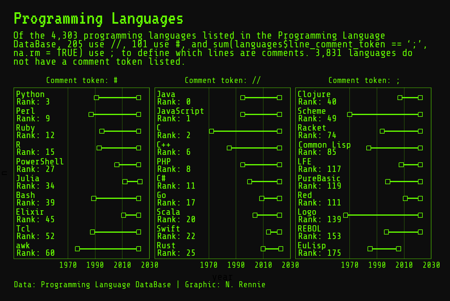
Chapter 2: Programming Languages Database
- Source: pldb.com (PLDB contributors 2022)
- License: PLDB content is published to the public domain and you can use it freely.
-
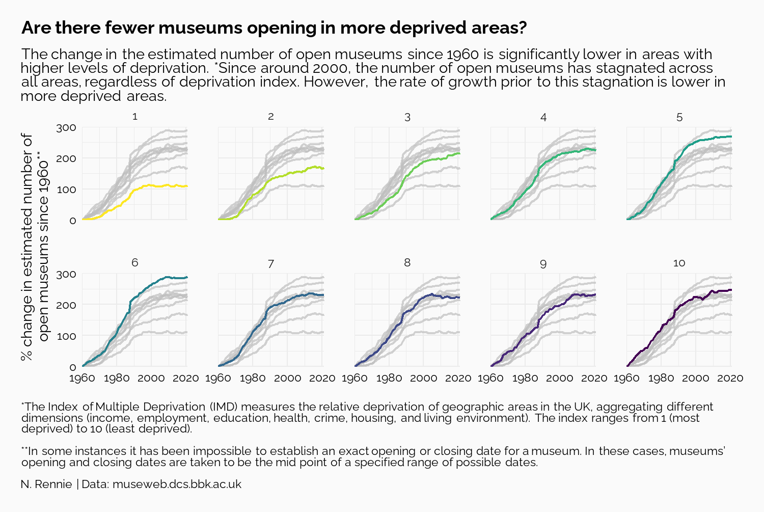
Chapter 3: Mapping Museums
- Source: museweb.dcs.bbk.ac.uk/allmus (Mapping Museums 2021)
- License: Licensed with Creative Commons Attribution 4.0 International.
-
Chapter 4: Honey Bee Colonies
- Source: usda.library.cornell.edu/concern/publications/rn301137d (United States Department of Agriculture: Economics, Statistics and Market Information System 2022)
- License: All publication files are considered government works and licensed with U.S. Public Domain.
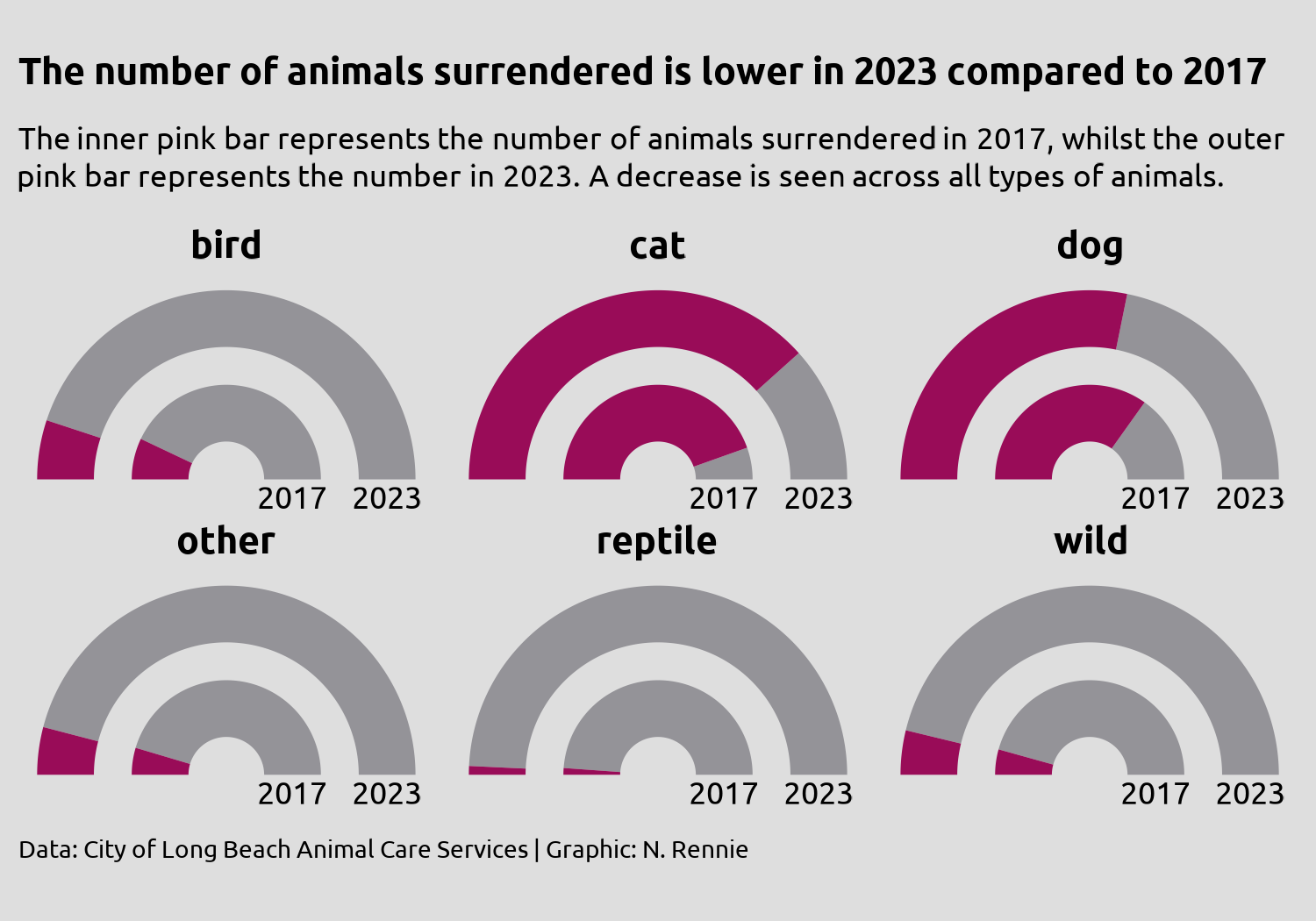
- Chapter 5: City of Long Beach Animal Shelter Data
-
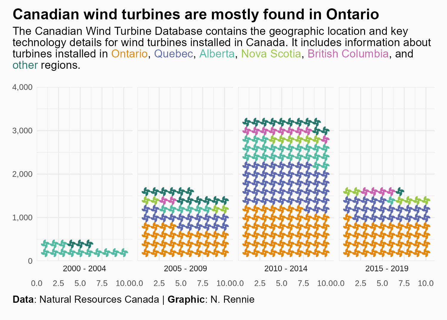
Chapter 6: Canadian Wind Turbine Database
- Source: open.canada.ca/data/en/dataset/79fdad93-9025-49ad-ba16-c26d718cc070 (Natural Resources Canada 2021)
- License: Licensed with Open Government Licence – Canada.
-
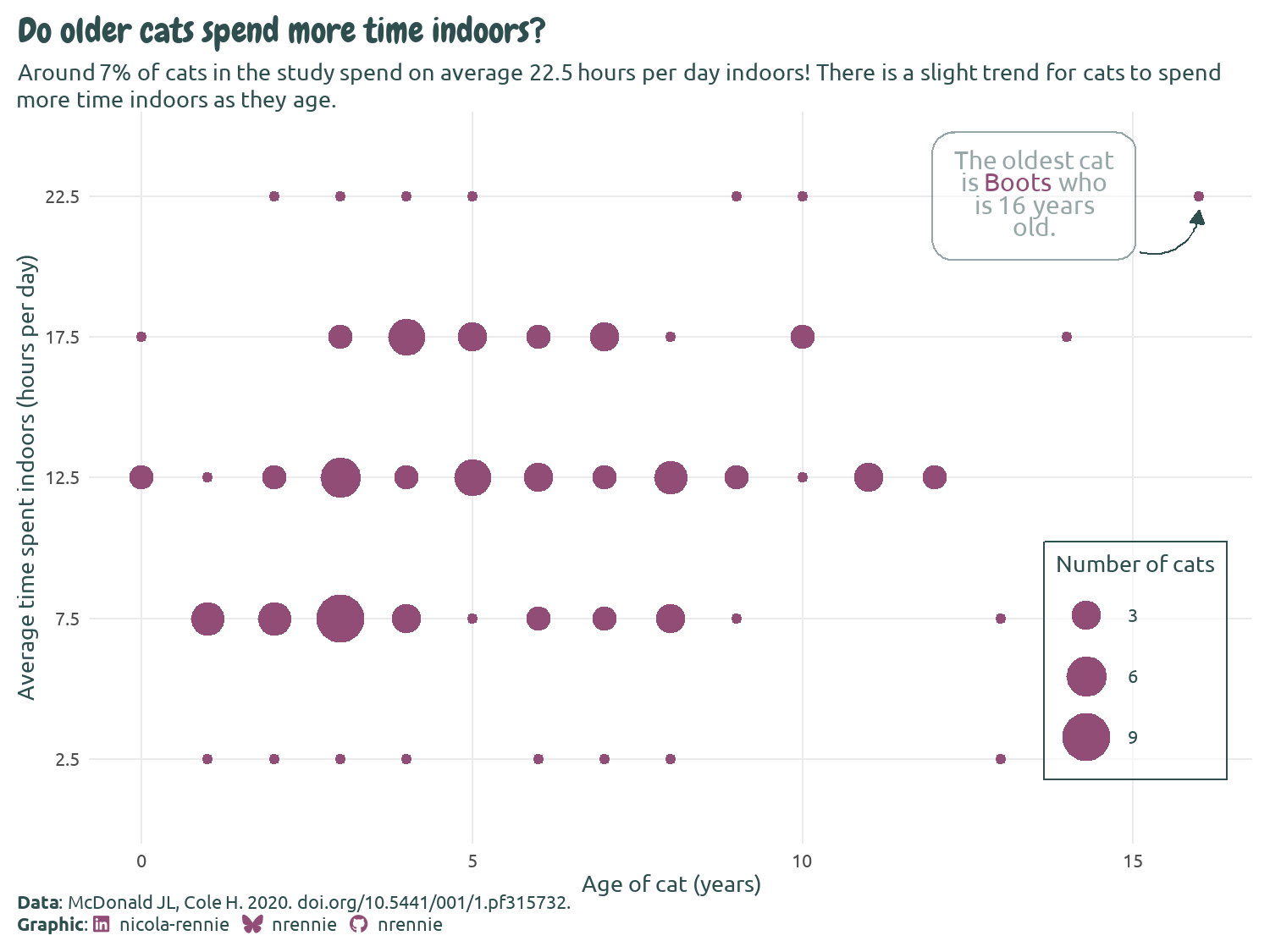
Chapter 7: The small home ranges and large local ecological impacts of pet cats
- Source: www.datarepository.movebank.org/entities/datapackage/4ef43458-a0c0-4ff0-aed4-64b07cedf11c (McDonald and Cole 2020)
- License: Licensed with Creative Commons Zero License.
-
Chapter 8: Nobel Prize Laureates
- Source: api.nobelprize.org/2.1/laureates (www.nobelprize.org 2024)
- License: Licensed with Creative Commons Zero License.
-
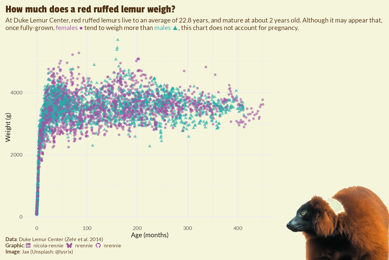
Chapter 9: Duke Lemur Center
- Source: lemur.duke.edu/duke-lemur-center-database (Zehr et al. 2014)
- License: Licensed with Creative Commons Zero License.
-
Chapter 10:
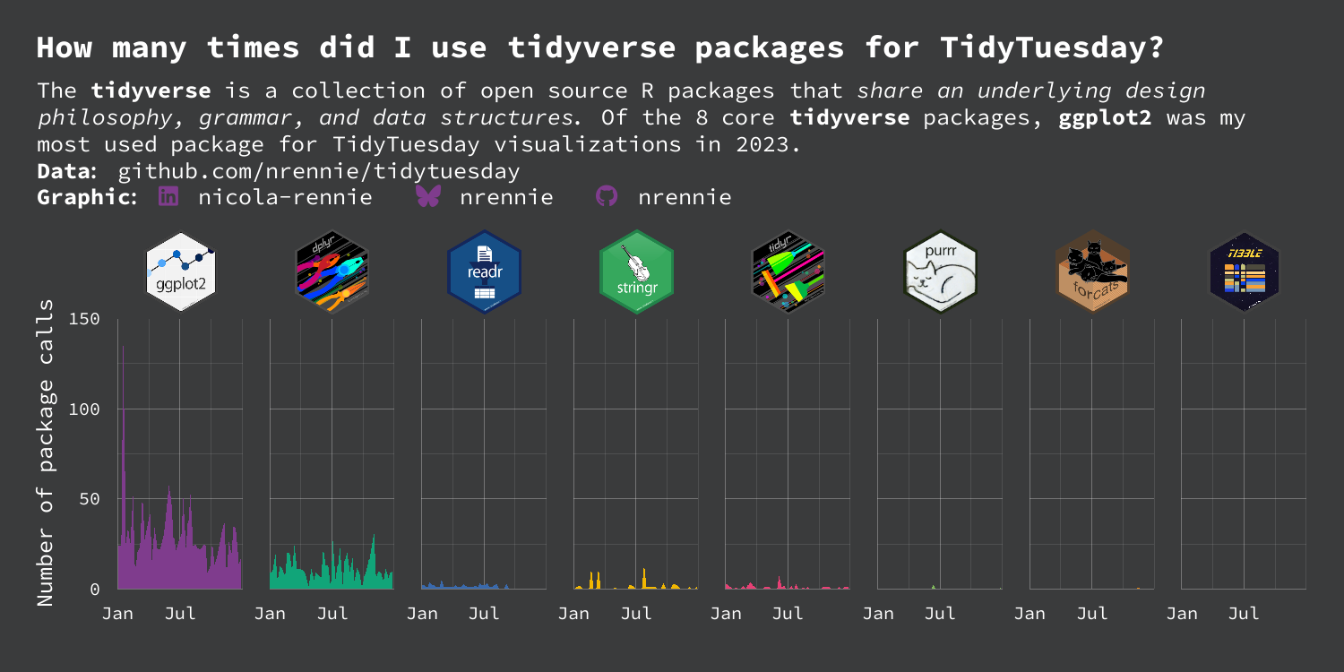
tidytuesdayGitHub Repository bynrennie- Source: github.com/nrennie/tidytuesday (Rennie 2024c)
- License: Licensed with Creative Commons Attribution 4.0 International.
-
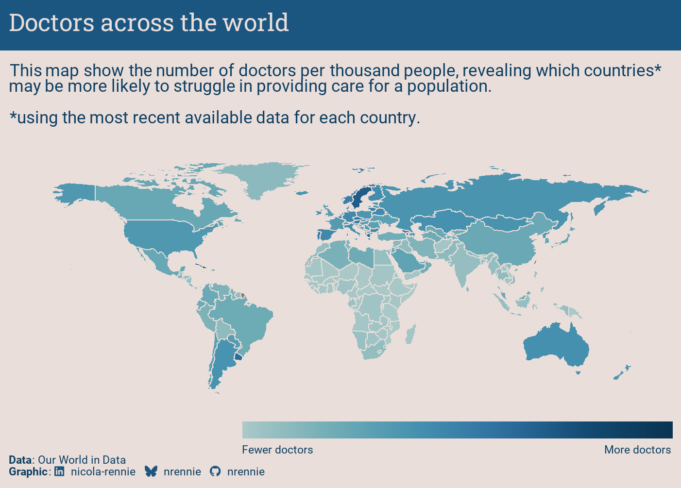
Chapter 11: Medical doctors per 1,000 people, 2019
- Source: ourworldindata.org/grapher/physicians-per-1000-people (Our World in Data 2019)
- License: Licensed with Creative Commons Attribution 4.0 International.
-
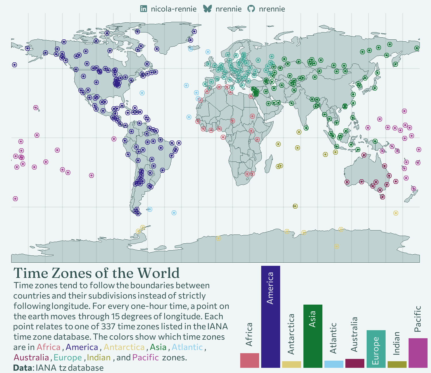
Chapter 12: Time Zones
- Source: data.iana.org/time-zones/tz-link.html#tzdb (Internet Assigned Numbers Authority 2023)
- License: This web page is in the public domain.
-
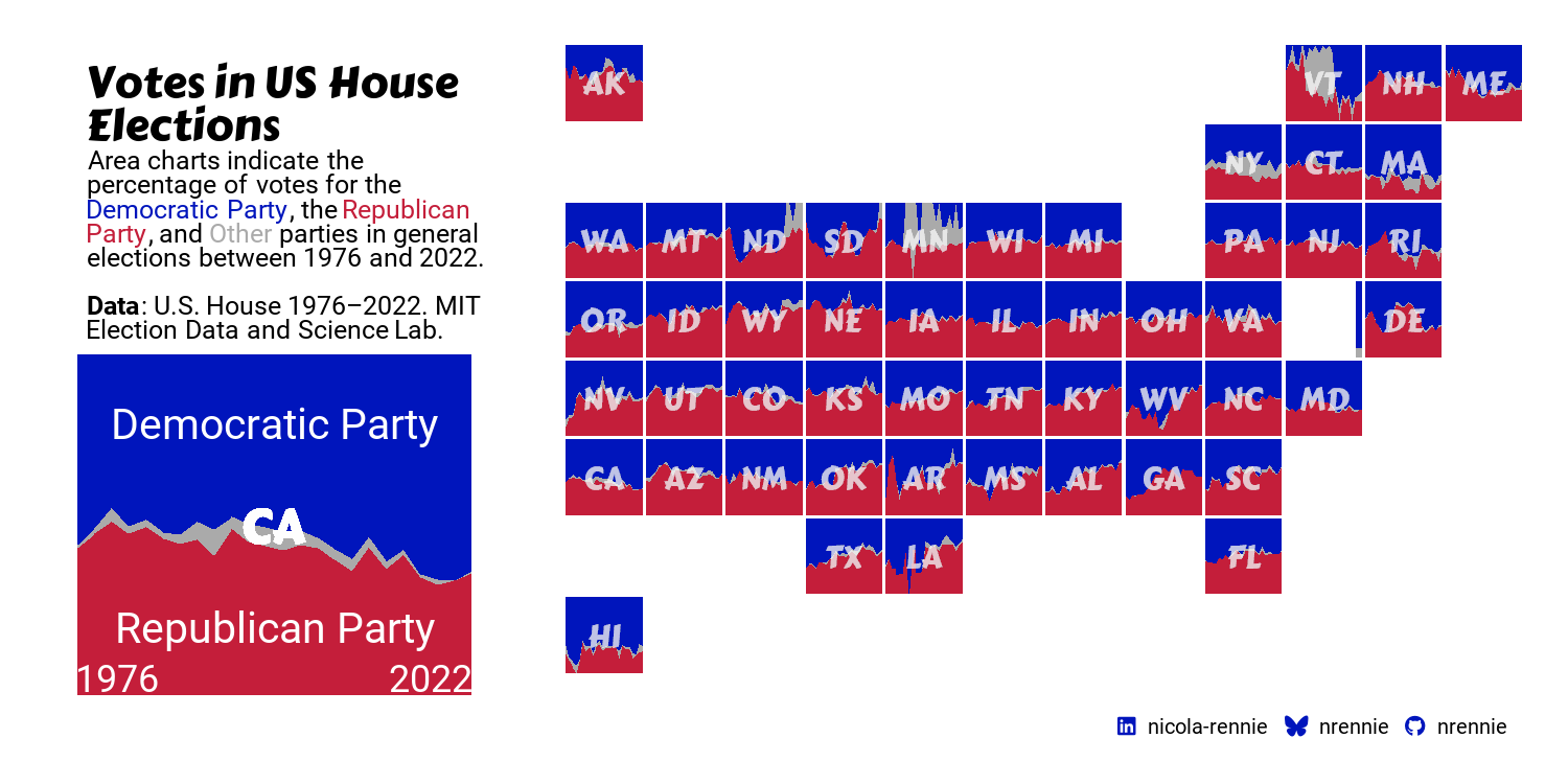
Chapter 13: US House Election Results
- Source: doi.org/10.7910/DVN/IG0UN2 (MIT Election Data and Science Lab 2017)
- License: Licensed with Creative Commons Zero License.
Images
All images used in this book (which were not created by the author) and links to the relevant licenses:
- Image: Lemur by Jax (@lysrix)
- Source: unsplash.com/photos/red-and-white-rodent-h5xrh3CNT-k (Jax (@lysrix) 2017)
- License: Licensed with Unsplash License.
- Image: {dplyr} Hex sticker
- Source: github.com/rstudio/hex-stickers/blob/main/PNG/dplyr.png (RStudio 2020a)
- License: Licensed with Creative Commons Zero License.
- Image: {ggplot2} Hex sticker
- Source: github.com/rstudio/hex-stickers/blob/main/PNG/gglot2.png (RStudio 2018b)
- License: Licensed with Creative Commons Zero License.
- Image: {tidyr} Hex sticker
- Source: github.com/rstudio/hex-stickers/blob/main/PNG/tidyr.png (RStudio 2020c)
- License: Licensed with Creative Commons Zero License.
- Image: {readr} Hex sticker
- Source: github.com/rstudio/hex-stickers/blob/main/PNG/readr.png (RStudio 2018d)
- License: Licensed with Creative Commons Zero License.
- Image: {purrr} Hex sticker
- Source: github.com/rstudio/hex-stickers/blob/main/PNG/purrr.png (RStudio 2018c)
- License: Licensed with Creative Commons Zero License.
- Image: {forcats} Hex sticker
- Source: github.com/rstudio/hex-stickers/blob/main/PNG/forcats.png (RStudio 2018a)
- License: Licensed with Creative Commons Zero License.
- Image: {tibble} Hex sticker
- Source: github.com/rstudio/hex-stickers/blob/main/PNG/tibble.png (RStudio 2018e)
- License: Licensed with Creative Commons Zero License.
- Image: {stringr} Hex sticker
- Source: github.com/rstudio/hex-stickers/blob/main/PNG/stringr.png (RStudio 2020b)
- License: Licensed with Creative Commons Zero License.
- Image: Wind Power Flaticon
- Source: www.flaticon.com/free-icon/wind-power_5670189 (Flaticon.com 2024)
- License: Licensed with Flaticon License: Free for personal and commercial purpose with attribution.
Visualization gallery
Chapter 2 Programming languages: dumbbell charts with ggplot2:
Chapter 3 UK museums: highlighting line charts with gghighlight:
Chapter 4 Bee colony losses: visualizing quantities with Poisson disk sampling:

Chapter 5 Animal shelter intakes: making gauge charts with ggforce:
Chapter 6 Canadian wind turbines: waffle plots and pictograms:
Chapter 7 Cats: data-driven annotations with ggtext:
Chapter 8 Nobel Prize laureates: positioning text and parameterizing plots:

Chapter 9 Lemurs: manipulating images in R:
Chapter 10 R packages: using images for custom facet labels:
 Chapter 11 Doctors across the world: making maps with ggplot2:
Chapter 12 Time zones: spatial data and mapping with sf:
 Chapter 13 US House elections: geography on a grid with geofacet:
Book cover
The (work-in-progress) cover of this book was also created with ggplot2. The code can be viewed below.
Code
# Packages ----------------------------------------------------------------

library(ggplot2)
library(showtext)
library(cropcircles)
library(ggimage)


# Fonts -------------------------------------------------------------------

font_add_google("Source Sans 3", "Source")
showtext_auto()
showtext_opts(dpi = 300)


# Functions ---------------------------------------------------------------

is_even <- function(x) {
  return((x %% 2) == 0)
}

make_hex_coords <- function(x0, y0, r) {
  angles <- seq(pi / 6, 2 * pi + pi / 6, length.out = 7)
  hexagon_coords <- function(xc, yc, rad, id) {
    x <- xc + rad * cos(angles)
    y <- yc + rad * sin(angles)
    data.frame(x = x, y = y, grp = id, x_grp = xc, y_grp = yc)
  }
  result <- do.call(
    rbind,
    mapply(hexagon_coords, x0, y0, r, seq_along(x0),
      SIMPLIFY = FALSE
    )
  )

  return(result)
}


# Parameters --------------------------------------------------------------

n_x <- 5
n_y <- 8

col_palette <- c("#FBEBFF", "#E999FF", "#9300B8", "#400052")
bg_col <- "#200029"
body_font <- "Source"

padding <- 20
width <- 5


# Generate data -----------------------------------------------------------

inputs <- expand.grid(
  x = seq(1, length.out = n_x, by = 1),
  y = seq(1, length.out = n_y, by = 1)
) |>
  tibble::as_tibble() |>
  dplyr::mutate(
    x = dplyr::if_else(
      is_even(y),
      x + 0.5,
      x
    )
  )
col_df <- data.frame(
  col_grp = seq(1, n_x + 0.5, by = 0.5),
  color = rev(grDevices::colorRampPalette(col_palette)(n_x * 2)),
  alpha = seq(0.2, 0.6, length.out = n_x * 2)
)
output <- make_hex_coords(
  x0 = inputs$x,
  y0 = inputs$y,
  r = rep(0.5, n_x * n_y)
) |>
  tibble::as_tibble() |>
  dplyr::left_join(col_df, by = c("x_grp" = "col_grp"))


# Subplots ----------------------------------------------------------------

g1 <- ggplot() +
  geom_col(
    data = data.frame(
      x = LETTERS[1:3],
      y = c(2, 5, 3)
    ),
    mapping = aes(x = x, y = y),
    fill = bg_col
  ) +
  theme_void() +
  theme(
    plot.background = element_rect(
      fill = "white", color = "white"
    ),
    axis.line.x.bottom = element_line(color = bg_col, linewidth = 1),
    axis.line.y.left = element_line(color = bg_col, linewidth = 1),
    plot.margin = margin(30, 30, 30, 30),
    aspect.ratio = 1
  )
tmp_a <- tempfile()
ggsave(tmp_a, g1,
       device = "png",
       height = 400, width = 400,
       dpi = 300, bg = bg_col,
       units = "px"
)
img_cropped_a <- crop_hex(tmp_a, bg_fill = "white")

set.seed(1234)
x <- runif(15)
g2 <- ggplot() +
  geom_point(
    data = data.frame(
      x = x,
      y = x + runif(15, 0, 0.1)
    ),
    mapping = aes(x = x, y = y),
    fill = bg_col
  ) +
  scale_x_continuous(limits = c(0, 1)) +
  scale_y_continuous(limits = c(0, 1)) +
  theme_void() +
  theme(
    plot.background = element_rect(
      fill = "white", color = "white"
    ),
    axis.line.x.bottom = element_line(color = bg_col, linewidth = 1),
    axis.line.y.left = element_line(color = bg_col, linewidth = 1),
    plot.margin = margin(30, 30, 30, 30),
    aspect.ratio = 1
  )
tmp_b <- tempfile()
ggsave(tmp_b, g2,
       device = "png",
       height = 400, width = 400,
       dpi = 300, bg = bg_col,
       units = "px"
)
img_cropped_b <- crop_hex(tmp_b, bg_fill = "white")

g3 <- ggplot() +
  geom_line(
    data = data.frame(
      x = 1:10,
      y = cumsum(runif(10))
    ),
    mapping = aes(x = x, y = y),
    color = bg_col
  ) +
  geom_line(
    data = data.frame(
      x = 1:10,
      y = cumsum(runif(10, 0, 0.5))
    ),
    mapping = aes(x = x, y = y),
    color = col_palette[3]
  ) +
  theme_void() +
  theme(
    plot.background = element_rect(
      fill = "white", color = "white"
    ),
    axis.line.x.bottom = element_line(color = bg_col, linewidth = 1),
    axis.line.y.left = element_line(color = bg_col, linewidth = 1),
    plot.margin = margin(30, 30, 30, 30),
    aspect.ratio = 1
  )
tmp_c <- tempfile()
ggsave(tmp_c, g3,
       device = "png",
       height = 400, width = 400,
       dpi = 300, bg = bg_col,
       units = "px"
)
img_cropped_c <- crop_hex(tmp_c, bg_fill = "white")


# Plot --------------------------------------------------------------------

ggplot() +
  geom_polygon(
    data = output,
    mapping = aes(
      x = x, y = y, group = grp,
      color = alpha(color, alpha)
    ),
    fill = "transparent",
    linewidth = 0.4
  ) +
  geom_image(
    data = output[1,],
    aes(
      x = 4.5,
      y = 4,
      image = img_cropped_a
    ),
    size = 0.1
  ) +
  geom_image(
    data = output[1,],
    aes(
      x = 2,
      y = 5,
      image = img_cropped_b
    ),
    size = 0.1
  ) +
  geom_image(
    data = output[1,],
    aes(
      x = 3.5,
      y = 6,
      image = img_cropped_c
    ),
    size = 0.1
  ) +
  annotate(
    "text",
    x = 1.25, y = 2.2,
    label = "The Art of Data\nVisualization\nwith ggplot2",
    family = body_font,
    color = "white",
    hjust = 0,
    vjust = 1,
    size = 28,
    fontface = "bold",
    size.unit = "pt"
  ) +
  annotate(
    "text",
    x = 1.25, y = 6.9,
    label = "Nicola Rennie",
    family = body_font,
    color = "white",
    hjust = 0,
    vjust = 1,
    size = 18,
    fontface = "bold",
    size.unit = "pt"
  ) +
  scale_color_identity() +
  scale_y_reverse() +
  coord_fixed(expand = FALSE, clip = "off") +
  theme_void() +
  theme(
    plot.background = element_rect(fill = bg_col, color = bg_col),
    plot.margin = margin(-padding, -padding, -padding, -padding)
  )


# Save --------------------------------------------------------------------

if (interactive()) {
  ggsave("images/cover.png",
         height = 1.5*width, width = width,
         dpi = 300, bg = bg_col
  )
}