Map of sexual orientation in Northern Ireland

Load required packages:

library(tidyverse)
library(ggview)
library(ggtext)
library(geojsonsf)
library(sf) # Needed for joining data

Prepare the data

Load the data:

sexual_age_ni <- read_csv("data/sexual_age_ni.csv")
ni_sf <- geojson_sf("data/spatial-data/osni_open_data_largescale_boundaries_local_government_districts_2012.geojson")

Prepare data for plotting:

plot_data <- sexual_age_ni |>
  filter(
    area_name != "Northern Ireland",
    age == "Usual residents aged 16 and over",
    sexual_orientation == "Gay, lesbian, bisexual, other sexual orientation"
  )

# Join to spatial data
map_data <- ni_sf |>
  select(LGDCode, geometry) |>
  left_join(plot_data, by = c("LGDCode" = "area_code"))

Plot preparation

Save colours as variables:

text_col <- "#ffffd9"
bg_col <- "#051338"

Tip

Use ggview to preview your plots at the desired size and resolution by adding the following to the end of your ggplot2 call:

+
  canvas(
    width = 5, height = 7,
    units = "in", bg = bg_col,
    dpi = 300
  )

Create the map

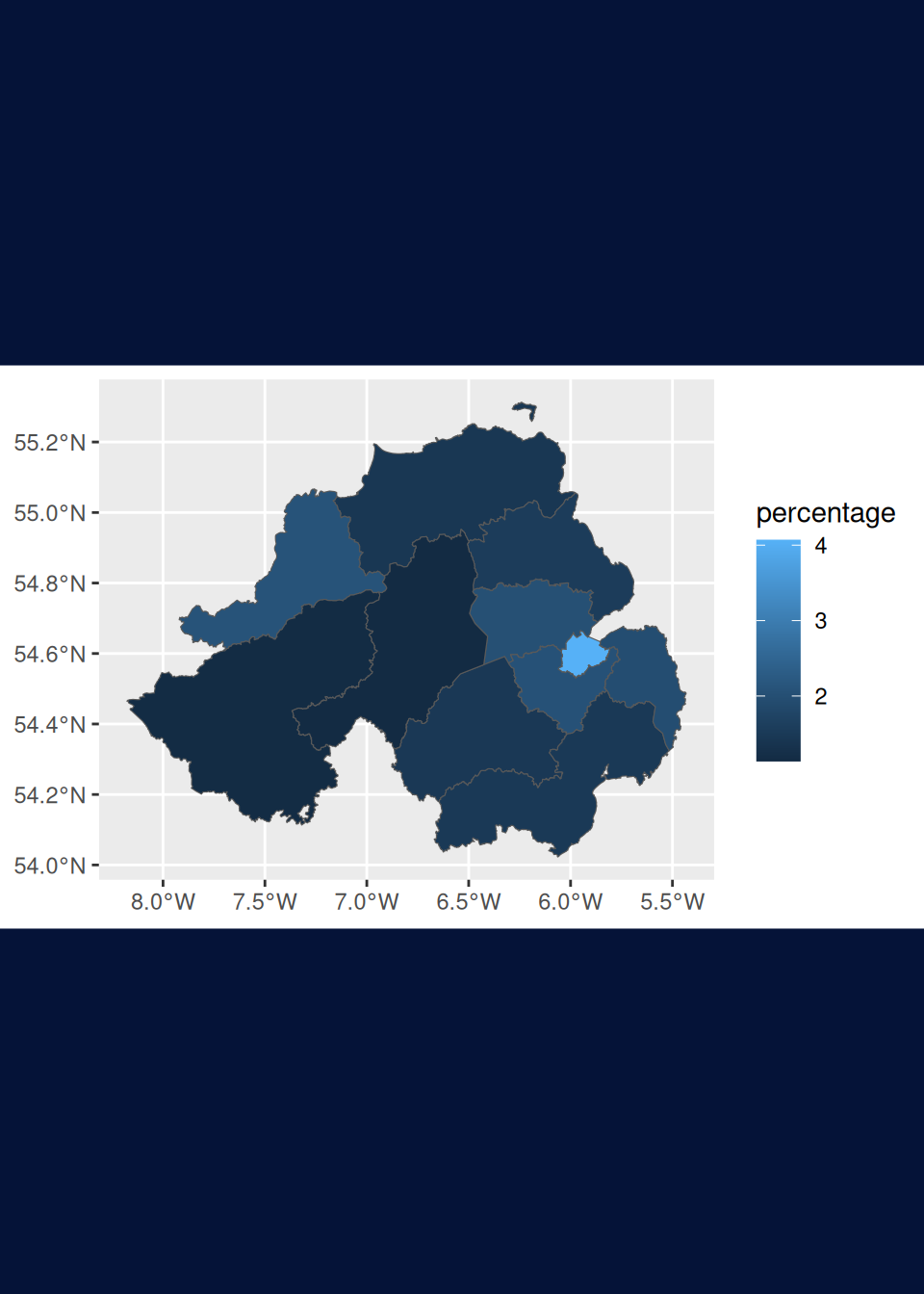
Version 1

ggplot() +
  geom_sf(
    data = map_data,
    mapping = aes(fill = percentage)
  )

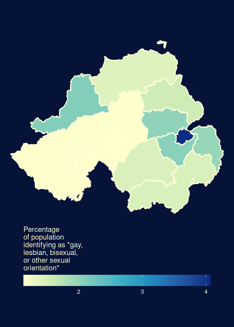
Version 2

ggplot() +
  geom_sf(
    data = map_data,
    mapping = aes(fill = percentage),
    colour = text_col,
    linewidth = 0.7
  ) +
  scale_fill_distiller(
    palette = "YlGnBu", direction = 1,
    name = str_wrap("Percentage of population identifying as *gay, lesbian, bisexual, or other sexual orientation*", 20)
  ) +
  theme_void() +
  theme(
    text = element_text(colour = text_col),
    legend.position = "bottom",
    legend.title.position = "top",
    legend.key.width = unit(4, "lines")
  ) 

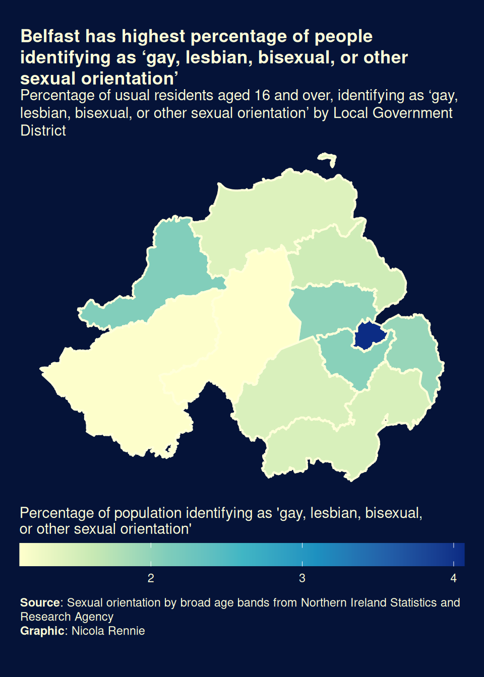
Version 3

ggplot() +
  geom_sf(
    data = map_data,
    mapping = aes(fill = percentage),
    colour = text_col,
    linewidth = 0.7
  ) +
  scale_fill_distiller(
    palette = "YlGnBu", direction = 1,
    name = str_wrap("Percentage of population identifying as 'gay, lesbian, bisexual, or other sexual orientation'", 65)
  ) +
  labs(
    title = "Belfast has highest percentage of people identifying as 'gay, lesbian, bisexual, or other sexual orientation'",
    subtitle = "Percentage of usual residents aged 16 and over, identifying as 'gay, lesbian, bisexual, or other sexual orientation' by Local Government District",
    caption = "**Source**: Sexual orientation by broad age bands from Northern Ireland Statistics and Research Agency<br>**Graphic**: Nicola Rennie"
  ) +
  theme_void() +
  theme(
    text = element_text(colour = text_col),
    legend.position = "bottom",
    legend.title.position = "top",
    legend.key.width = unit(4.6, "lines"),
    plot.title.position = "plot",
    plot.caption.position = "plot",
    plot.title = element_textbox_simple(face = "bold", margin = margin(b = 15)),
    plot.subtitle = element_textbox_simple(margin = margin(b = 5)),
    plot.caption = element_textbox_simple(margin = margin(t = 10)),
    plot.margin = margin(10, 15, 10, 15)
  )

Save the plot

ggsave("map.png",
  bg = bg_col,
  height = 7, width = 5
)

If you’ve used ggview, then assign the plot to a variable e.g. p and then do:

save_ggplot(
  plot = p,
  file = "map.png"
)