Five ggplot2 functions I wish I’d known about earlier

There are a few small tweaks you can make to your ggplot2 code to improve your charts. However, they’re not often mentioned. So here’s a few functions and arguments I wish I’d known about earlier.

In order to make a chart effective, aesthetic, and accessible, you will almost always need to adjust the default styling - regardless of which programming language or packages you use. In ggplot2 there are lots of helpful functions and arguments that massively improve how your chart looks. However, a lot of these functions aren’t taught or don’t come up in examples very often. And so many of us (myself included) learn the hard way to do things, and then later find out we could have just changed one argument to do all of it! So this blog post will explain five ggplot2 functions that I wish I’d known about earlier!

We’ll start by loading the packages we need for some examples, including ggplot2 of course! We’ll use the gapminder package for some data, and dplyr to do a little bit of data wrangling.

library(ggplot2)
library(gapminder)
library(dplyr)

Warning

The example charts used in this blog post have deliberately had minimal styling applied to keep the code simple and demonstrate one feature at a time. That means many of the examples may not be the best looking chart, and would require a little bit more work before being of publication quality!

guide_axis()

When creating faceted plots, you’ll often find that the axis text gets squashed due to the reduced space available. For example, in this faceted line chart of life expectancy over time, the x-axis labels for the years overlap, making them very hard to read.

plot_data <- gapminder |>
  filter(continent == "Americas")
g <- ggplot(
  data = plot_data,
  mapping = aes(x = year, y = lifeExp)
) +
  geom_line() +
  facet_wrap(~country)
g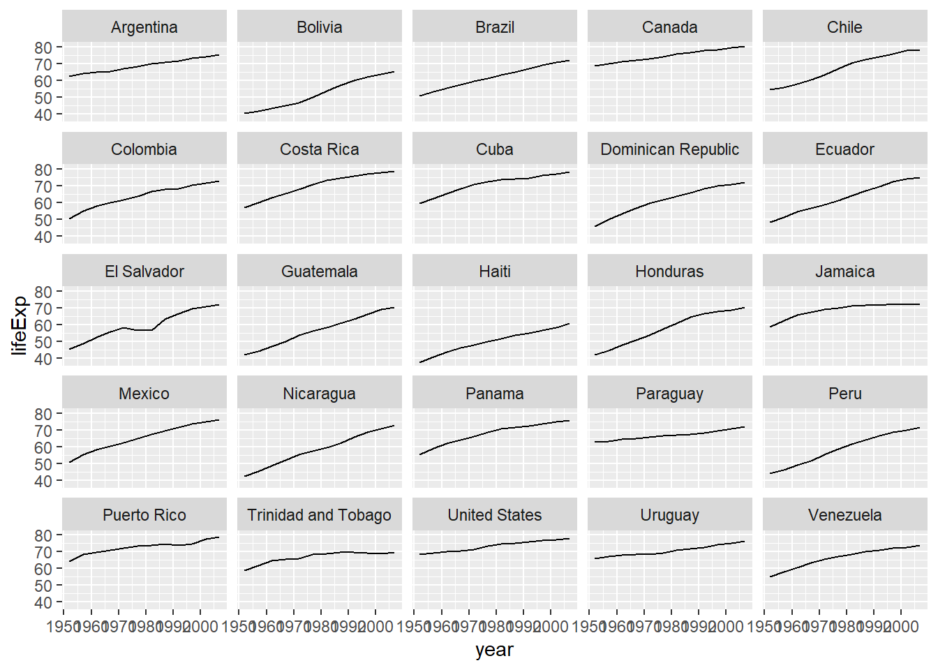

You could manually adjust the breaks and labels, but there’s an easier way. Within scale_x_continuous() you can adjust the axis using the guide_axis() function for the guide argument. We don’t often think about x and y variables as having a guide (i.e., legend) but that’s essentially what an axis is. It helps to think about x and y variables in the same way as colour and fill. In guide_axis(), there’s an argument called check.overlap. By default, this argument is FALSE. If it’s TRUE, it will silently remove overlapping labels, while prioritising keeping the first, last, and middle labels.

g + scale_x_continuous(
  guide = guide_axis(check.overlap = TRUE)
)

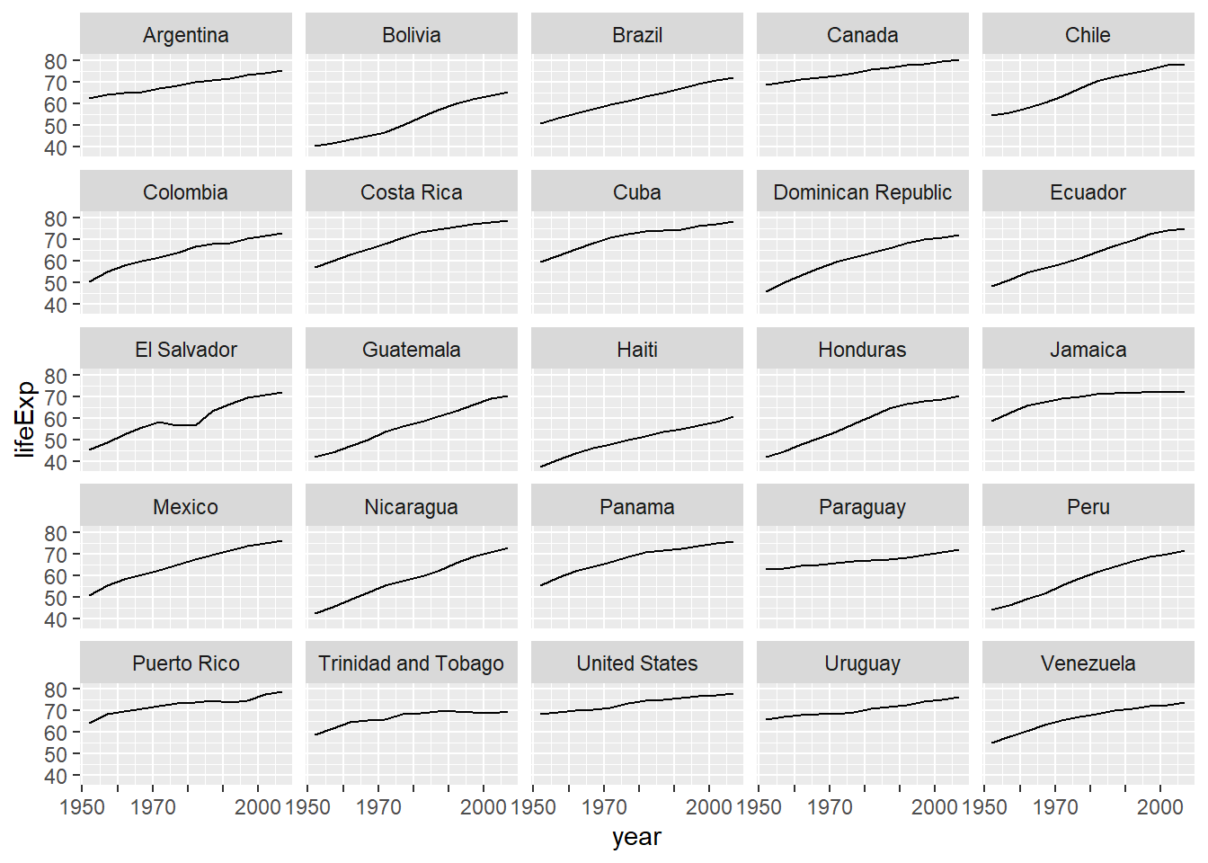
With one extra line of code, the chart looks so much cleaner and easier to read!

size_unit

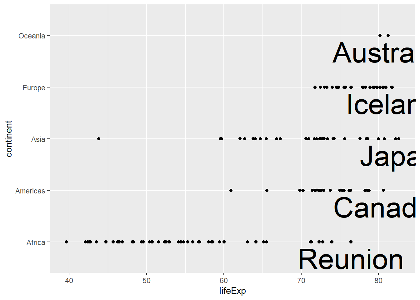
If you’ve ever added some labels or annotations using geom_text() and tried to adjust the text size, you might have been confused by the text sizing. For example, if you want to make the text a little bit bigger, you might set the size argument to 12, which results in huge labels!

plot_data <- gapminder |>
  filter(year == 2007)
text_data <- plot_data |>
  group_by(continent) |>
  slice_max(lifeExp) |>
  ungroup()
g <- ggplot() +
  geom_point(
    data = plot_data,
    mapping = aes(x = lifeExp, y = continent)
  )

g +
  geom_text(
    data = text_data,
    mapping = aes(x = lifeExp, y = continent, label = country),
    vjust = 1.3,
    size = 12, # make the text a little bit bigger
  )

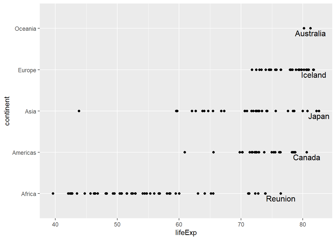
The default font size in geom_text() is 3.88 which might seem like an unusual value! This is because the default unit for geom_text() is millimetres rather than the more common points (pts), which is used within theme(). Instead of trying to convert millimetres to points, you can simply changed the units used, making it easier to use consistent font sizes between the theme and annotations.

g +
  geom_text(
    data = text_data,
    mapping = aes(x = lifeExp, y = continent, label = country),
    vjust = 1.3,
    size = 12,
    size.unit = "pt"
  )

rel()

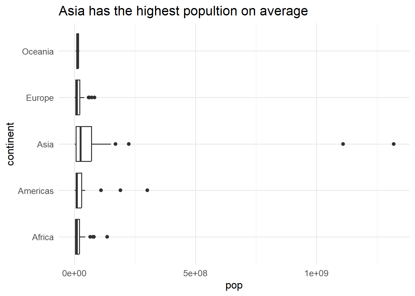
Since dealing with fonts in R is often tricky, here’s another text sizing tip! Let’s say we want to increase the font size across all chart elements. We can do this within any of the theme_*() functions, using the base_size argument. We might also want to further increase the size of the title text, and can use the size argument element_text() to do that.

plot_data <- gapminder |>
  filter(year == 2007)
g <- ggplot(
  data = plot_data,
  mapping = aes(x = pop, y = continent)
) +
  geom_boxplot() +
  labs(title = "Asia has the highest popultion on average")

g +
  theme_minimal(base_size = 13) +
  theme(
    plot.title = element_text(size = 16)
  )

This plot looks perfectly fine. However, a problem might arise if we need to resize the chart and increase or decrease the font size. This would mean going through every function and argument where we’ve specified a text size and updating to new values. This is a bit tedious, and prone to errors. Instead, we can specify relative font sizes using the rel() function. This means the title text will be 1.25 times larger than the base size.

g +
  theme_minimal(base_size = 13) +
  theme(
    plot.title = element_text(size = rel(1.25))
  )

It looks the same as the previous plot, but it’s much easier to make adjustments. Now if we need to change the text size across the entire chart, we can simple update the base_size argument and everything else will be resized accordingly.

plot.title.position

If you’ve ever added a title to a plot, especially a chart where you have long y-axis category labels, you may notice that the title isn’t positioned at the left hand side of the plot. To demonstrate this, let’s make a simple bar chart of GDP per capita in different countries in 1952. You can see that the title is neither left aligned nor centre aligned within the chart. Instead, it’s hovering in a slightly weird place.

plot_data <- gapminder |>
  filter(continent == "Americas", year == 1952)
g <- ggplot(
  data = plot_data,
  mapping = aes(x = gdpPercap, y = country)
) +
  geom_col() +
  labs(title = "GDP per capita")
g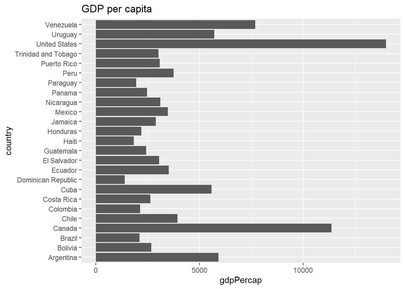

We can fix this by using the theme() function, and setting the argument plot.title.position to "plot". By default, this argument is set to "panel" which aligns the text with the plot panel (the grey area, which might not be visible with a different theme). Setting it to "plot" aligns the text to the whole plot.

g +
  theme(
    plot.title.position = "plot"
  )

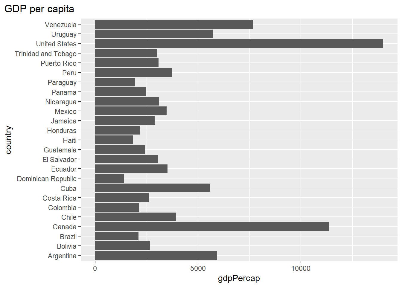
This looks much cleaner and professional, and means you can use all of the space available for longer titles or subtitles!

Tip

Setting plot.title.position adjusts both the title and subtitle. If you also want to adjust the caption, the plot.caption.position argument works similarly.

bg

When styling a chart, it’s very common to change the theme. This might be to a different built-in theme, one from another R package, or one of your own design. What might not be immediately obvious is that some themes have a white background, whereas others have a transparent background.

g +
  theme_minimal() +
  theme(
    plot.title.position = "plot"
  )
ggsave("barchart.png", width = 5, height = 4)

You might not notice that the background is transparent, as many documents and slides also have white backgrounds. However, you may see something like this , if you open the image.

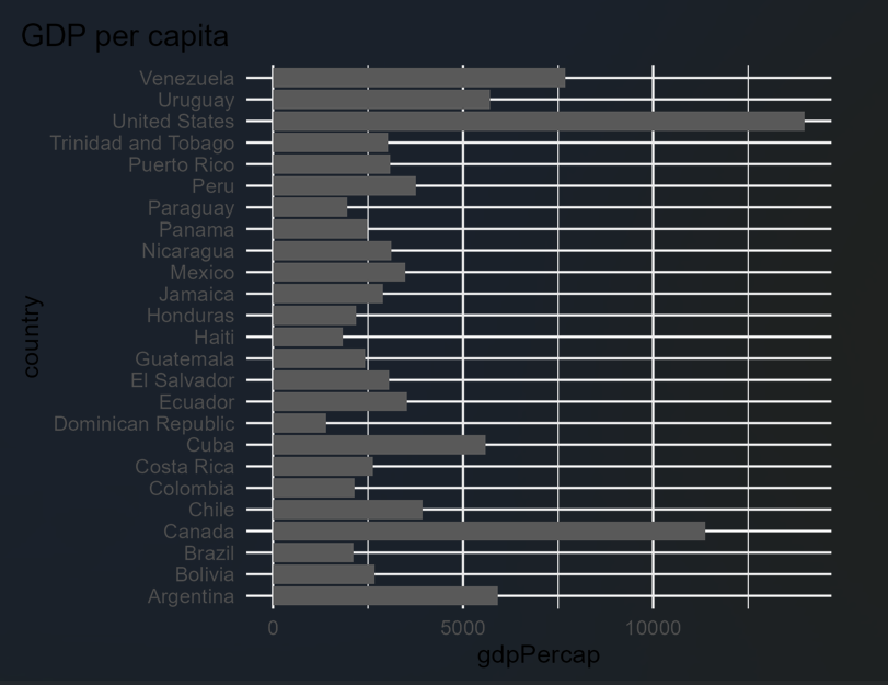
We can fix this when saving, by adding a colour to the bg argument of ggsave() which adjusts the background colour.

ggsave(
  "barchart.png", width = 5, height = 4,
  bg = "white"
)

Warning

Since version 4.0.0 of ggplot2, the ways that background colours can be adjusted have changed. Now, all theme_*() functions, have a paper argument. The default for theme_minimal() is now "white". This might cause some unexpected issues if (like me) you were relying on the default being transparent!

Bonus: scale_x/y_symmetric()

This helpful function isn’t actually in ggplot2 itself, so it’s included as a bonus! For continuous variables, the default axis range is simply the range of the data. However if you’re plotting data that has a skewed distribution, where the middle of the data isn’t in the middle of the range, this can make it harder to see that the data is skewed. This is especially true when comparing differences above or below 0, for example. To demonstrate, here’s a scatter plot of the difference in a country’s life expectancy from the average across all countries.

plot_data <- gapminder |>
  filter(year == 2007) |>
  mutate(lifeExpDiff = lifeExp - mean(lifeExp))
g <- ggplot(
  data = plot_data,
  mapping = aes(x = continent, y = lifeExpDiff)
) +
  geom_point(position = position_jitter(height = 0, width = 0.3))
g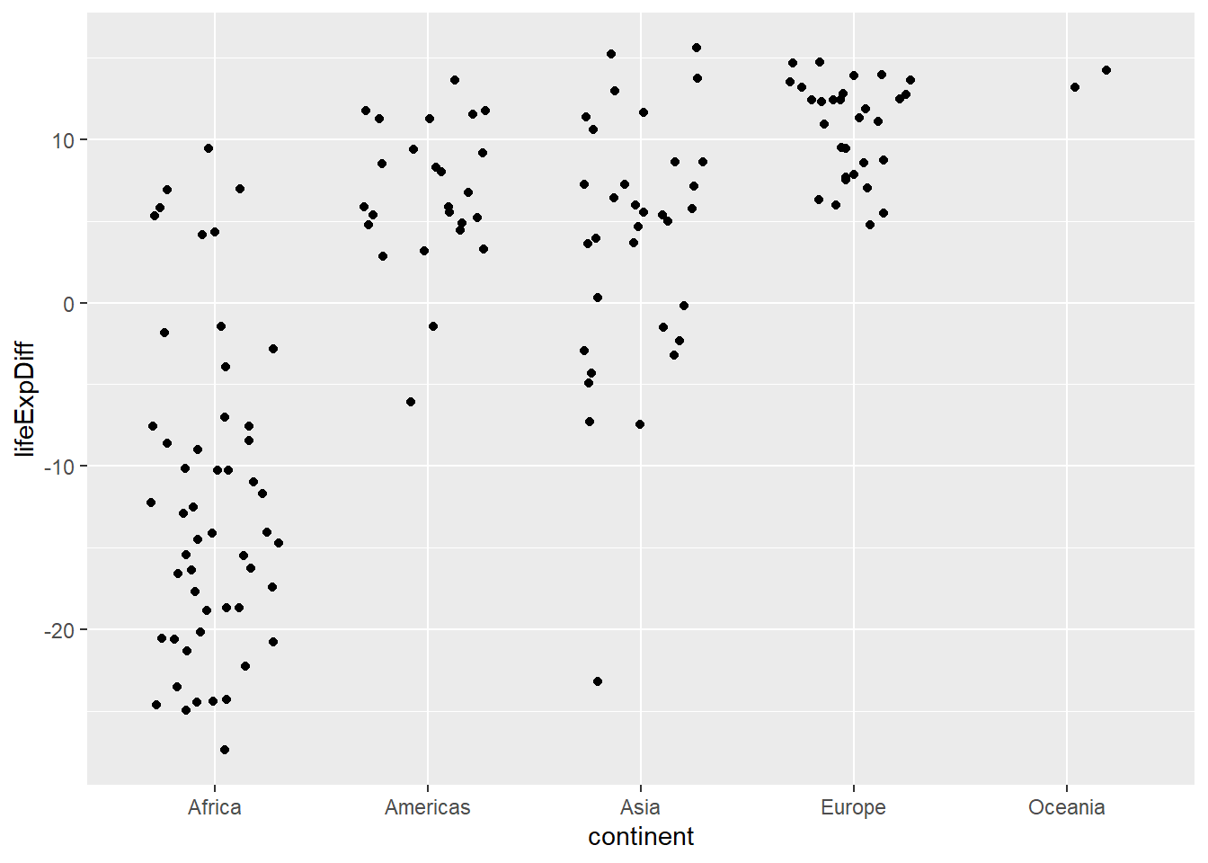

If you look carefully at the chart, you’ll notice that most of the values are less than 0. However, at first glance, the chart might suggest that it is equally spread above and below zero because we often expect 0 to be in the middle of the chart. But it isn’t. Of course, you can calculate the limits of the data and pass in the absolute maximum (with positive and negative values) to the limits argument of the scale_y_continuous() function. An easier way to fix this, is to use scale_y_symmetric() from the lemon package.

library(lemon)
g +
  scale_y_symmetric()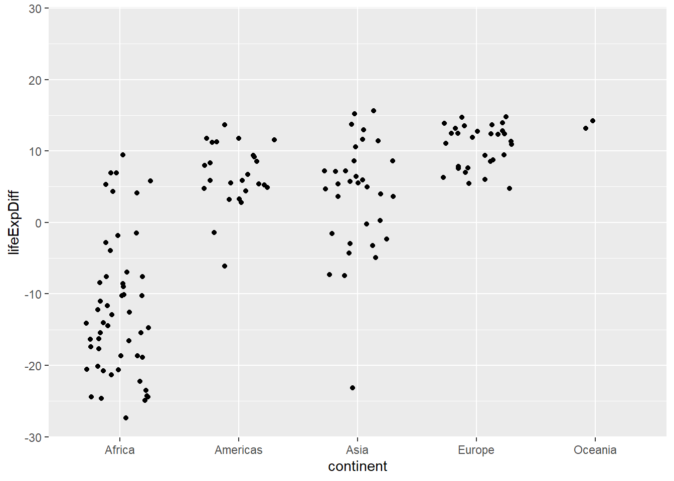

This is especially useful for residuals plots where you’re often comparing the spread above and below 0.

Tip

The analogous function for the x axis is scale_x_symmetric(). You can adjust the mid point using the mid argument if you need to show whether something is symmetric about some value other than 0.

TipMore ggplot2 resources

• The Art of Data Visualization with ggplot2: nrennie.rbind.io/art-of-viz

• ggplot2: Elegant Graphics for Data Analysis: ggplot2-book.org

• R Graphics Cookbook: r-graphics.org