age <- c(15, 25, 32, 87, 12)Exercises
Data
Hypoxia MAP Treatment Dataset
The Hypoxia MAP dataset was contributed by Dr. Amy Nowacki, Associate Professor, Cleveland Clinic. Please refer to this resource as: Amy S. Nowacki, “Hypoxia MAP Treatment Dataset”, TSHS Resources Portal (2022). Available at causeweb.org/tshs/hypoxia. The data is licensed under a Creative Commons Attribution-Non Commerical-Share Alike 4.0 International (CC BY-NC-SA 4.0) license, and is intended for educational purposes only.
Download CSV: hypoxia.csv
Download Excel: hypoxia.xlsx
Note:
Female- 0 = male
- 1 = female
Race- 1 = African American
- 2 = Caucasian
- 3 = Other
Type Surg- 1 = gastroenterostomy
- 2 = gastric restrictive procedure
- 3 = gastroplasty
- 4 = removal of gastric restrictive device
Exercises
Exercise 1: Performing operations in R
- Create a vector called
age(like the one below). Multiply each element by 5.
Solution
age * 5[1] 75 125 160 435 60- What does the
sqrt()function do? Apply thesqrt()function to each element ofage.
Solution
sqrt(age)[1] 3.872983 5.000000 5.656854 9.327379 3.464102- Install the {ggplot2} package.
Solution
install.packages("ggplot2")- Load the {ggplot2} package into R.
Solution
library(ggplot2)Exercise 2: Loading data into R
- Make an R project file (File –> New Project). Download either the CSV or Excel file of the Hypoxia data from the section below and save it into your R project folder. Load the data into R.
Solution
You can use read.csv():
hypoxia <- read.csv("data/hypoxia.csv")But the read_csv() function from {readr} is a little bit nicer:
library(readr)
hypoxia <- read_csv("data/hypoxia.csv")
For Excel files
library(readxl)Warning: package 'readxl' was built under R version 4.4.3hypoxia <- read_xlsx("data/hypoxia.xlsx")- Inspect the data using
View().
Solution
View(hypoxia)- How many rows and columns are in the data?
Solution
nrow(hypoxia)[1] 281ncol(hypoxia)[1] 36- Create a summary of the data.
Solution
summary(hypoxia) Age Female Race BMI
Min. :16.40 Min. :0.0000 Min. :1.000 Min. :23.40
1st Qu.:39.60 1st Qu.:0.0000 1st Qu.:2.000 1st Qu.:41.50
Median :48.20 Median :1.0000 Median :2.000 Median :46.00
Mean :47.29 Mean :0.7153 Mean :1.826 Mean :46.75
3rd Qu.:54.70 3rd Qu.:1.0000 3rd Qu.:2.000 3rd Qu.:51.70
Max. :73.80 Max. :1.0000 Max. :3.000 Max. :71.70
Sleeptime Min Sao2 AHI Smoking
Min. : 0.00 Min. :28.00 Min. :1.000 Min. :0.0000
1st Qu.: 1.40 1st Qu.:74.00 1st Qu.:2.000 1st Qu.:0.0000
Median : 8.10 Median :82.00 Median :3.000 Median :1.0000
Mean :18.71 Mean :78.71 Mean :2.871 Mean :0.5018
3rd Qu.:26.90 3rd Qu.:86.00 3rd Qu.:4.000 3rd Qu.:1.0000
Max. :99.60 Max. :95.00 Max. :4.000 Max. :1.0000
NA's :3
Diabetes Hyper CAD Preop AntiHyper Med
Min. :0.0000 Min. :0.0000 Min. :0.00000 Min. :0.0000
1st Qu.:0.0000 1st Qu.:0.0000 1st Qu.:0.00000 1st Qu.:0.0000
Median :0.0000 Median :1.0000 Median :0.00000 Median :0.0000
Mean :0.3452 Mean :0.7082 Mean :0.09253 Mean :0.2384
3rd Qu.:1.0000 3rd Qu.:1.0000 3rd Qu.:0.00000 3rd Qu.:0.0000
Max. :1.0000 Max. :1.0000 Max. :1.00000 Max. :1.0000
CPAP Type Surg Duration of Surg Duration of Surg1
Min. :0.0000 Min. :1.000 Min. :2.000 Min. :0.2000
1st Qu.:0.0000 1st Qu.:1.000 1st Qu.:3.700 1st Qu.:0.4000
Median :1.0000 Median :1.000 Median :4.200 Median :0.5000
Mean :0.6335 Mean :1.224 Mean :4.315 Mean :0.5131
3rd Qu.:1.0000 3rd Qu.:1.000 3rd Qu.:4.900 3rd Qu.:0.6000
Max. :1.0000 Max. :4.000 Max. :7.900 Max. :1.1000
NA's :6
Duration of Surg2 TWA MAP TWA MAP1 TWA MAP2
Min. :1.400 Min. : 66.00 Min. : 51.96 Min. : 66.17
1st Qu.:3.000 1st Qu.: 81.24 1st Qu.: 70.70 1st Qu.: 82.76
Median :3.500 Median : 88.55 Median : 78.02 Median : 89.73
Mean :3.552 Mean : 89.01 Mean : 79.24 Mean : 90.30
3rd Qu.:4.100 3rd Qu.: 95.94 3rd Qu.: 86.40 3rd Qu.: 98.16
Max. :7.000 Max. :127.20 Max. :111.10 Max. :132.71
NA's :3 NA's :4
TWA HR TWA HR1 TWA HR2 Intraop AntiHyper Med
Min. : 54.22 Min. : 50.32 Min. : 53.61 Min. :0.0000
1st Qu.: 68.89 1st Qu.: 66.28 1st Qu.: 68.52 1st Qu.:0.0000
Median : 75.38 Median : 73.98 Median : 75.89 Median :0.0000
Mean : 76.10 Mean : 75.58 Mean : 76.14 Mean :0.3096
3rd Qu.: 82.91 3rd Qu.: 83.48 3rd Qu.: 83.61 3rd Qu.:1.0000
Max. :109.09 Max. :124.59 Max. :105.25 Max. :1.0000
NA's :78 NA's :82 NA's :78
Vasopressor Ephedrine Ephedrine Amt Epinephrine
Min. :0.0000 Min. :0.0000 Min. : 0.000 Min. :0.000000
1st Qu.:0.0000 1st Qu.:0.0000 1st Qu.: 0.000 1st Qu.:0.000000
Median :1.0000 Median :0.0000 Median : 0.000 Median :0.000000
Mean :0.5445 Mean :0.3452 Mean : 5.196 Mean :0.007117
3rd Qu.:1.0000 3rd Qu.:1.0000 3rd Qu.:10.000 3rd Qu.:0.000000
Max. :1.0000 Max. :1.0000 Max. :50.000 Max. :1.000000
Epinephrine Amt Phenylephrine Phenylephrine Amt MAC
Min. :0.000e+00 Min. :0.0000 Min. :0.0000 Min. :0.510
1st Qu.:0.000e+00 1st Qu.:0.0000 1st Qu.:0.0000 1st Qu.:2.080
Median :0.000e+00 Median :0.0000 Median :0.0000 Median :2.830
Mean :7.117e-05 Mean :0.3879 Mean :0.1232 Mean :2.841
3rd Qu.:0.000e+00 3rd Qu.:1.0000 3rd Qu.:0.1000 3rd Qu.:3.410
Max. :1.000e-02 Max. :1.0000 Max. :2.5700 Max. :6.560
NA's :1
Propofol Induction IV Morphine Eq Crystalloids Colloids
Min. : 0.0 Min. : 6.70 Min. : 400 Min. : 0.0
1st Qu.:200.0 1st Qu.: 25.00 1st Qu.:2400 1st Qu.: 0.0
Median :200.0 Median : 30.30 Median :3000 Median : 500.0
Mean :206.9 Mean : 43.43 Mean :2994 Mean : 482.4
3rd Qu.:250.0 3rd Qu.: 40.00 3rd Qu.:3500 3rd Qu.:1000.0
Max. :400.0 Max. :1101.10 Max. :6950 Max. :2000.0
Exercise 3: Plotting single variables
- Create a histogram of the age of all patients in the study. What does the
binsargument ingeom_histogram()do?
Solution
Load ggplot2:
library(ggplot2)ggplot(
data = hypoxia,
mapping = aes(x = Age)
) +
geom_histogram()`stat_bin()` using `bins = 30`. Pick better value with `binwidth`.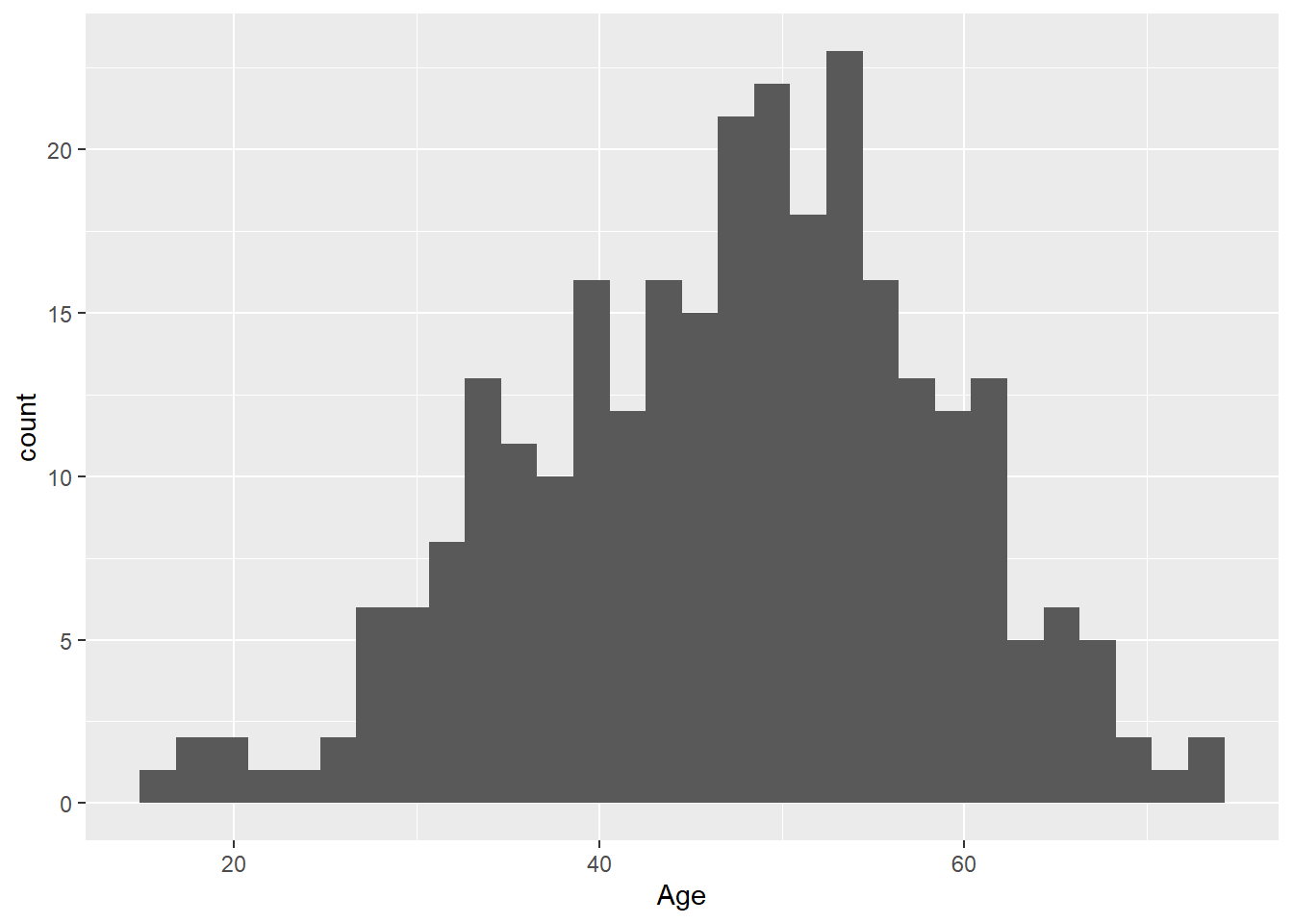
Choose a different number of bins with bins:
ggplot(
  data = hypoxia,
  mapping = aes(x = Age)
) +
  geom_histogram(bins = 20)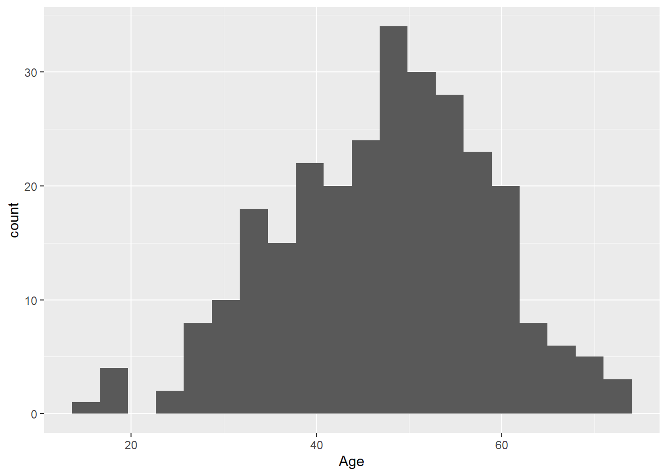
- Create a histogram of the age of all female patients in the study. Hint: remember that 0 = male and 1 = female in the
Femalecolumn.
Solution
library(dplyr)
# Filter data to only females
f_hypoxia <- hypoxia %>%
  filter(Female == 1)
# Plot histogram
ggplot(
  data = f_hypoxia,
  mapping = aes(x = Age)
) +
  geom_histogram()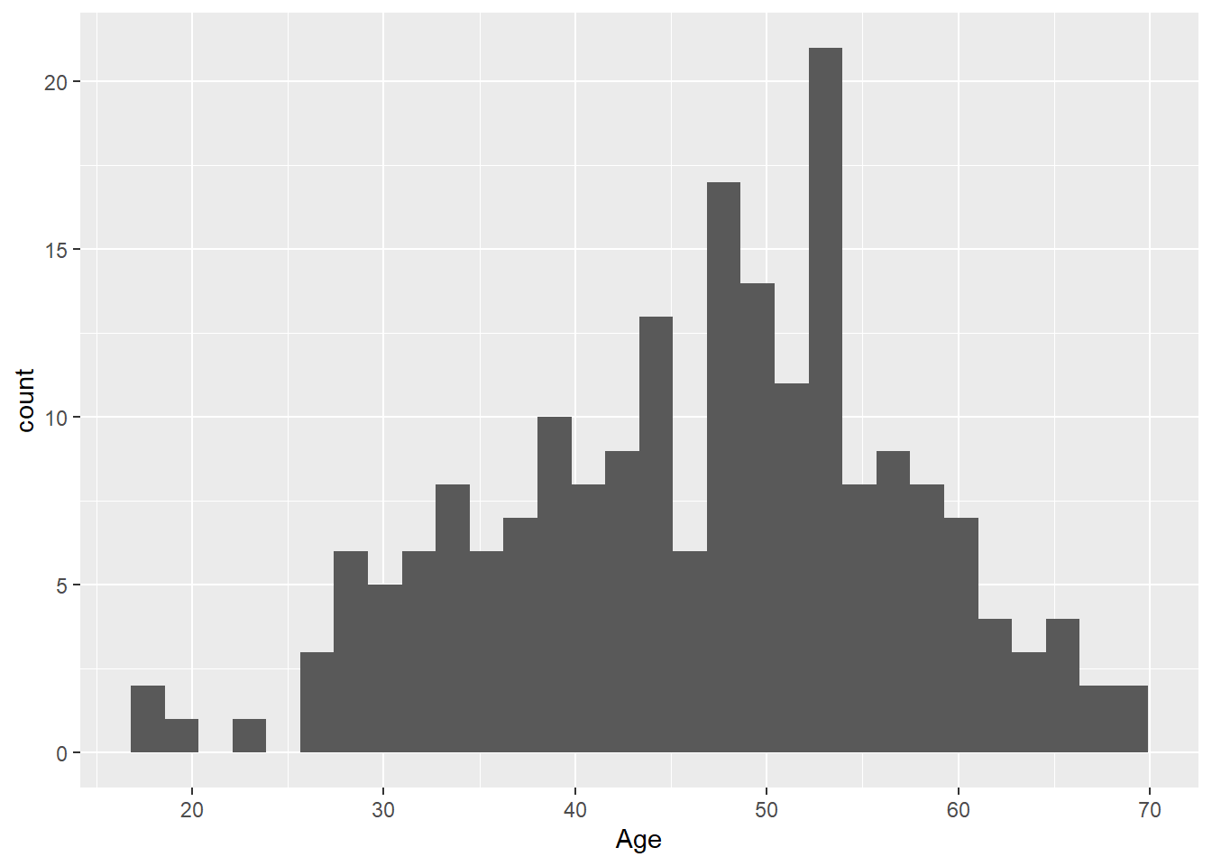
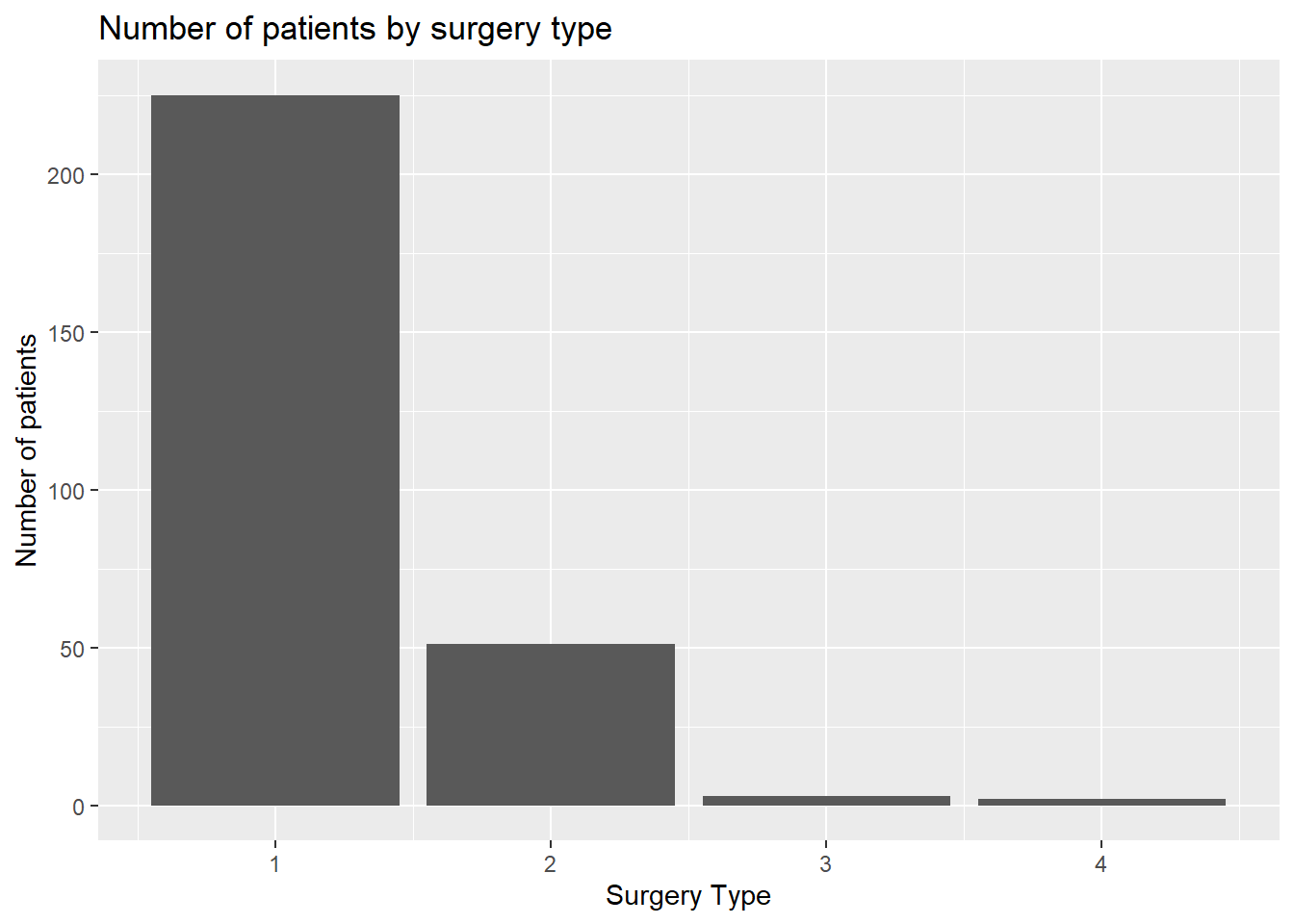
- Create a bar chart of the number of people who had each surgery type. Hint:
geom_bar().
Solution
ggplot(
  data = hypoxia,
  mapping = aes(x = `Type Surg`)
) +
  geom_bar()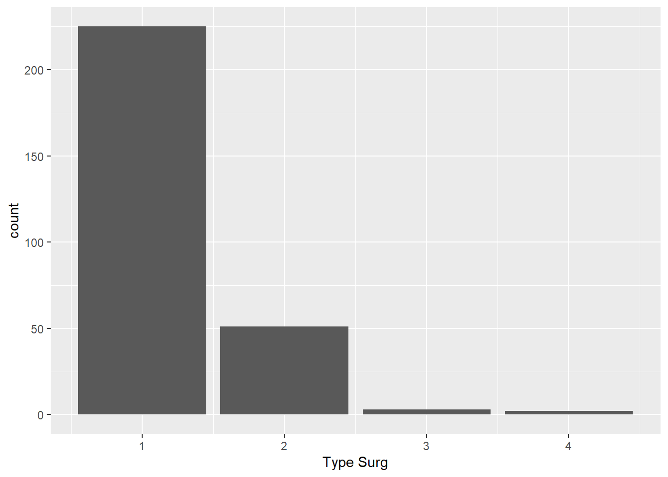
- Bonus: Edit the axis labels using the
labs()function. Can you also add a title?
Solution
ggplot(
  data = hypoxia,
  mapping = aes(x = `Type Surg`)
) +
  geom_bar() +
  labs(
    x = "Surgery Type", y = "Number of patients",
    title = "Number of patients by surgery type"
  )
Exercise 4: Reading help files in R
- The {ggplot2} package is often used for plotting in R. What does the
geom_count()function do?
Hint: use the
?and try the examples!
Solution
?geom_countThe geom_count() function creates a bubble plot where the size of the points is proportional to the number of observations at each unique x and y combination.
- What is the difference between
geom_bar()andgeom_col()?
Solution
?geom_bargeom_bar()counts the number of observations of a categorical variable and puts the count on the y-axis (i.e. R does the counting for you)geom_col()puts the values in a column on the y-axis (i.e. you do the counting)
- Does this code do what you expect? Can you fix it?
ggplot(
  data = hypoxia,
  mapping = aes(x = `Type Surg`, fill = "blue")
) +
  geom_bar()
Solution
ggplot(
  data = hypoxia,
  mapping = aes(x = `Type Surg`)
) +
  geom_bar(fill = "blue")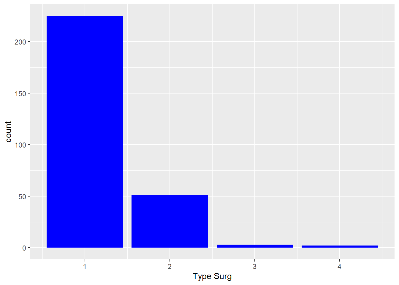
- the
fillargument changes the colour inside the bars - the colour isn’t mapped to a column in the data so it shouldn’t be inside the
aes()function.
Exercise 5: Plotting multiple variables
- Create a scatter plot of age (on the x-axis) and BMI (on the y-axis).
Solution
ggplot(
  data = hypoxia,
  mapping = aes(x = Age, y = BMI)
) +
  geom_point()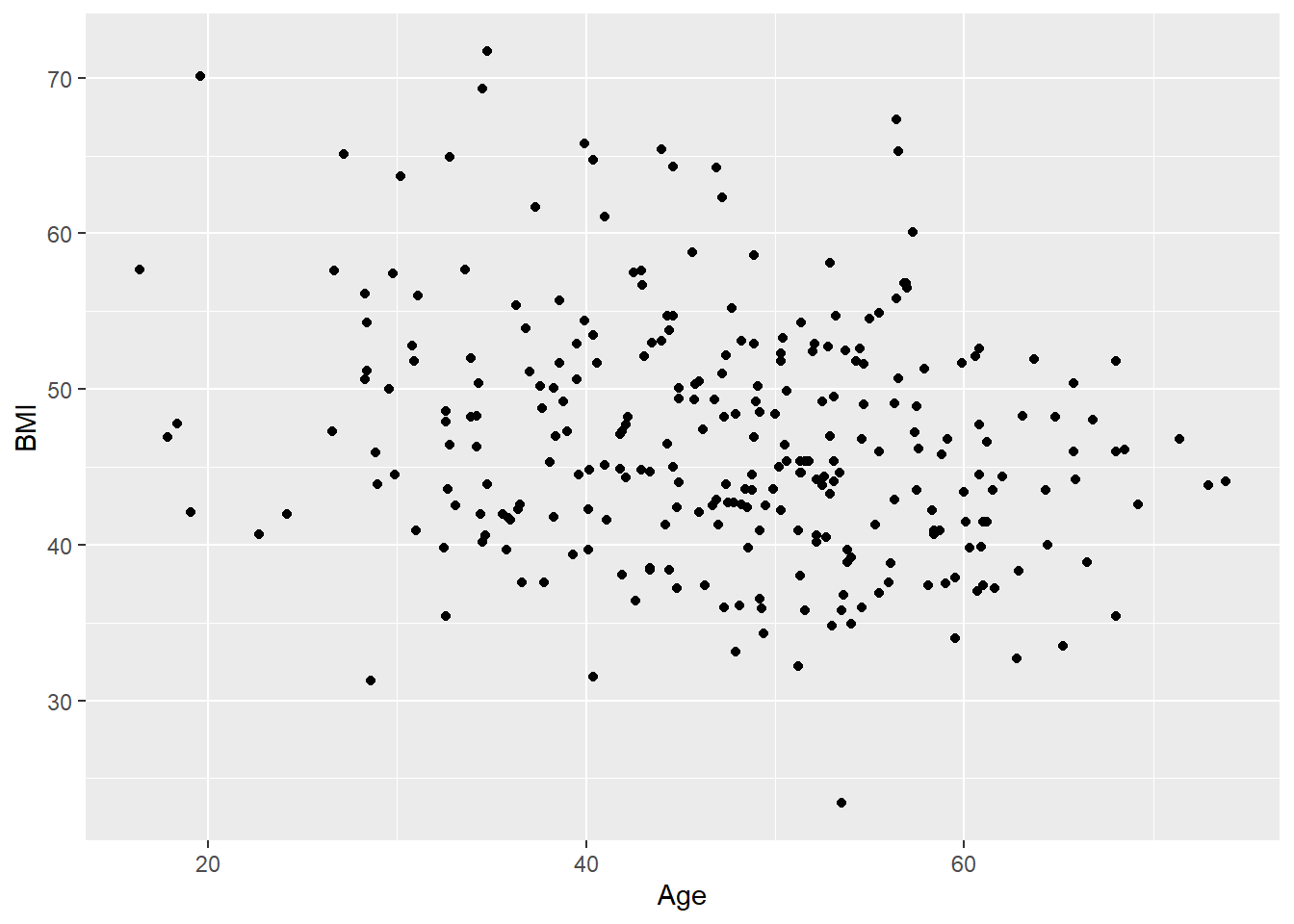
- Create a boxplot of age for each surgery type. Hint: make
`Type Surg`afactor().
Solution
ggplot(
  data = hypoxia,
  mapping = aes(x = Age, y = factor(`Type Surg`))
) +
  geom_boxplot()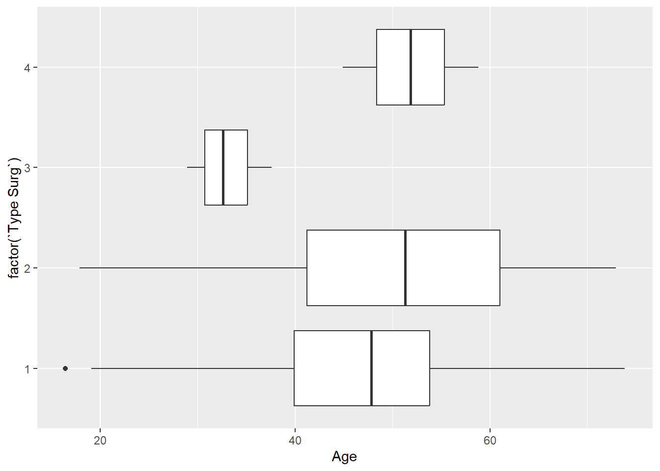
- Create a bar chart of the number of people who had each surgery type. Colour the bars based on whether people had diabetes. Hint: should
Diabetesbe a numeric or a factor?
Solution
ggplot(
  data = hypoxia,
  mapping = aes(x = `Type Surg`, fill = factor(Diabetes))
) +
  geom_bar()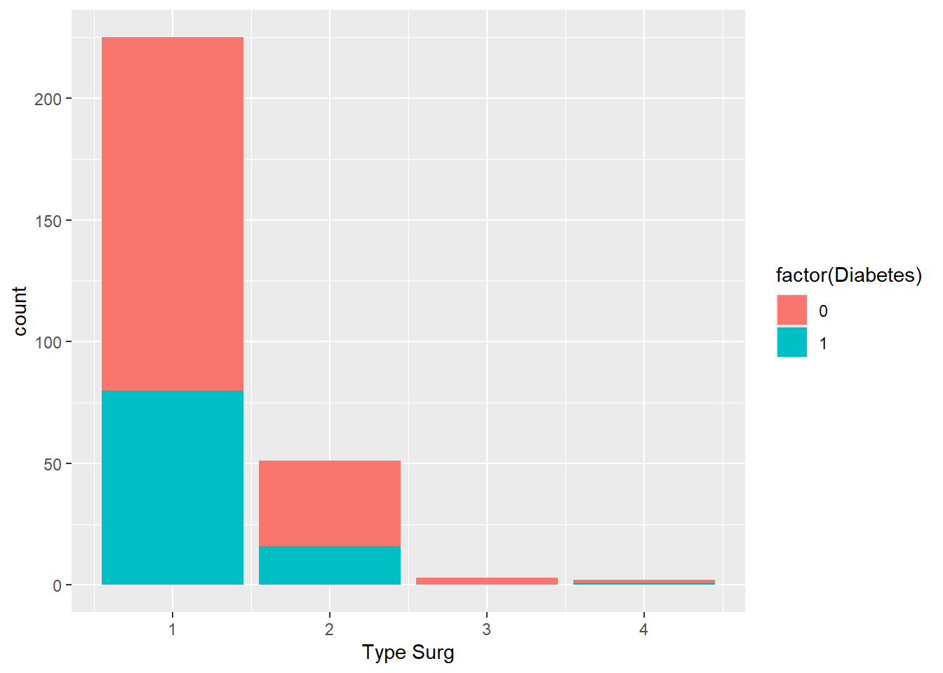
- Bonus: Edit your bar chart to put the bars next to each other instead of stacked on top. Hint: look at the
positionargument ingeom_bar().
Solution
ggplot(
  data = hypoxia,
  mapping = aes(x = `Type Surg`, fill = factor(Diabetes))
) +
  geom_bar(position = position_dodge())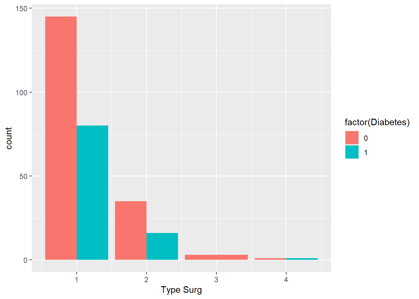
Note that the bar for Type 3 surgery is twice as wide because there are no people with diabetes who had this surgery. To fix this:
ggplot(
  data = hypoxia,
  mapping = aes(x = `Type Surg`, fill = factor(Diabetes))
) +
  geom_bar(position = position_dodge(preserve = "single"))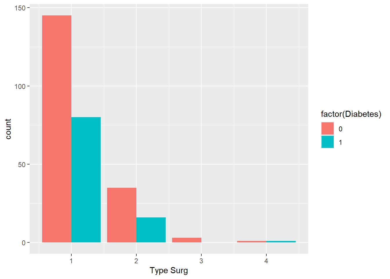
Exercise 6: Computing summary statistics
- For each of the columns
`Duration of Surg`andAHI, calculate the following summary statistics: mean and standard deviation.
If there are any missing values, calculate the mean of the non-missing values. Hint: Look at the na.rm argument for ?mean.
Solution
Using the summarise() function:
hypoxia %>%
  summarise(
    mean_dur = mean(`Duration of Surg`),
    mean_ahi = mean(AHI),
    sd_dur = sd(`Duration of Surg`),
    sd_ahi = sd(AHI),
  )
# A tibble: 1 × 4
mean_dur mean_ahi sd_dur sd_ahi
<dbl> <dbl> <dbl> <dbl>
1 4.31 NA 1.12 NAExclude missing values from the calculation:
hypoxia %>%
  summarise(
    mean_dur = mean(`Duration of Surg`),
    mean_ahi = mean(AHI, na.rm = TRUE),
    sd_dur = sd(`Duration of Surg`),
    sd_ahi = sd(AHI, na.rm = TRUE),
  )
# A tibble: 1 × 4
mean_dur mean_ahi sd_dur sd_ahi
<dbl> <dbl> <dbl> <dbl>
1 4.31 2.87 1.12 1.08- Repeat the calculations, but group the summary statistics by Surgery Type (
`Type Surg`).
Solution
hypoxia %>%
  group_by(`Type Surg`) %>%
  summarise(
    mean_dur = mean(`Duration of Surg`),
    mean_ahi = mean(AHI, na.rm = TRUE),
    sd_dur = sd(`Duration of Surg`),
    sd_ahi = sd(AHI, na.rm = TRUE),
  )
# A tibble: 4 × 5
`Type Surg` mean_dur mean_ahi sd_dur sd_ahi
<dbl> <dbl> <dbl> <dbl> <dbl>
1 1 4.61 2.92 0.928 1.04
2 2 2.91 2.75 0.640 1.21
3 3 4.57 1.67 0.808 0.577
4 4 6.7 2.5 1.41 2.12 - Bonus: also calculate the median, minimum, and maximum.
Solution
hypoxia %>%
  group_by(`Type Surg`) %>%
  summarise(
    mean_dur = mean(`Duration of Surg`),
    mean_ahi = mean(AHI, na.rm = TRUE),
    sd_dur = sd(`Duration of Surg`),
    sd_ahi = sd(AHI, na.rm = TRUE),
    median_dur = median(`Duration of Surg`),
    median_ahi = median(AHI, na.rm = TRUE),
    min_dur = min(`Duration of Surg`),
    min_ahi = min(AHI, na.rm = TRUE),
    max_dur = max(`Duration of Surg`),
    max_ahi = max(AHI, na.rm = TRUE),
  )
# A tibble: 4 × 11
`Type Surg` mean_dur mean_ahi sd_dur sd_ahi median_dur median_ahi min_dur
<dbl> <dbl> <dbl> <dbl> <dbl> <dbl> <dbl> <dbl>
1 1 4.61 2.92 0.928 1.04 4.4 3 2.9
2 2 2.91 2.75 0.640 1.21 2.8 3 2
3 3 4.57 1.67 0.808 0.577 4.1 2 4.1
4 4 6.7 2.5 1.41 2.12 6.7 2.5 5.7
# ℹ 3 more variables: min_ahi <dbl>, max_dur <dbl>, max_ahi <dbl>Exercise 7: Summary tables
- Create a descriptive table of patient characteristics, which includes the following variables: age, gender, race, smoking.
Solution
library(gtsummary)Warning: package 'gtsummary' was built under R version 4.4.3tbl1_data <- hypoxia %>%
select(Age, Female, Race, Smoking)
tbl1_data %>%
tbl_summary()| Characteristic | N = 2811 |
|---|---|
| Age | 48 (40, 55) |
| Female | 201 (72%) |
| Race | |
| 1 | 57 (20%) |
| 2 | 216 (77%) |
| 3 | 8 (2.8%) |
| Smoking | 141 (50%) |
| 1 Median (Q1, Q3); n (%) | |
- Are
FemaleandSmokingrepresented in the table in a way that makes sense? Change theFemaleandSmokingcolumns to afactor. Hint: you might want to look at themutate()function to edit the columns in the data.
Solution
tbl1_data %>%
  mutate(
    Smoking = factor(Smoking),
    Female = factor(Female)
  ) %>%
tbl_summary()| Characteristic | N = 2811 |
|---|---|
| Age | 48 (40, 55) |
| Female | |
| 0 | 80 (28%) |
| 1 | 201 (72%) |
| Race | |
| 1 | 57 (20%) |
| 2 | 216 (77%) |
| 3 | 8 (2.8%) |
| Smoking | |
| 0 | 140 (50%) |
| 1 | 141 (50%) |
| 1 Median (Q1, Q3); n (%) | |
- Group the table by
Smoking.
Hint: look at the
byargument intbl_summary().
Solution
tbl1_data %>%
  mutate(
    Smoking = factor(Smoking),
    Female = factor(Female)
  ) %>%
tbl_summary(by = Smoking)| Characteristic | 0 N = 1401 |
1 N = 1411 |
|---|---|---|
| Age | 45 (35, 53) | 51 (44, 57) |
| Female | ||
| 0 | 35 (25%) | 45 (32%) |
| 1 | 105 (75%) | 96 (68%) |
| Race | ||
| 1 | 29 (21%) | 28 (20%) |
| 2 | 106 (76%) | 110 (78%) |
| 3 | 5 (3.6%) | 3 (2.1%) |
| 1 Median (Q1, Q3); n (%) | ||
- Bonus: Change the labels for
SmokingtoSmokingandNo smokinginstead of1and0.
Solution
tbl1_data %>%
  mutate(
    Smoking = factor(Smoking,
      levels = c(0, 1),
      labels = c("No smoking", "Smoking")
    ),
    Female = factor(Female)
  ) %>%
tbl_summary(Smoking)| Characteristic | No smoking N = 1401 |
Smoking N = 1411 |
|---|---|---|
| Age | 45 (35, 53) | 51 (44, 57) |
| Female | ||
| 0 | 35 (25%) | 45 (32%) |
| 1 | 105 (75%) | 96 (68%) |
| Race | ||
| 1 | 29 (21%) | 28 (20%) |
| 2 | 106 (76%) | 110 (78%) |
| 3 | 5 (3.6%) | 3 (2.1%) |
| 1 Median (Q1, Q3); n (%) | ||
Exercise 8: Statistical tests
- Perform a t-test to test whether the age of patients is significantly different for males and females. Assume the variances of the two groups are equal.
Solution
# Subset data
f_hypoxia <- filter(hypoxia, Female == 1)
m_hypoxia <- filter(hypoxia, Female == 0)

# Unpaired t-test
t.test(f_hypoxia$Age, m_hypoxia$Age, var.equal = TRUE)
    Two Sample t-test

data:  f_hypoxia$Age and m_hypoxia$Age
t = -1.9334, df = 279, p-value = 0.0542
alternative hypothesis: true difference in means is not equal to 0
95 percent confidence interval:
 -5.70622115  0.05134553
sample estimates:
mean of x mean of y
46.48756 49.31500 - Test if the variances of the two groups are actually equal.
Solution
var.test(f_hypoxia$Age, m_hypoxia$Age)
    F test to compare two variances

data:  f_hypoxia$Age and m_hypoxia$Age
F = 0.78536, num df = 200, denom df = 79, p-value = 0.1829
alternative hypothesis: true ratio of variances is not equal to 1
95 percent confidence interval:
 0.5341363 1.1205117
sample estimates:
ratio of variances
         0.7853552