Examples

Data

Length of Stay Model Data

The LOS dataset is a simulated hospital length-of-stay dataset, available through the {NHSRdatasets} R package. The dataset is licensed under creativecommons.org/publicdomain/zero/1.0.

Download CSV: LOS.csv

Download Excel: LOS.xlsx

If you have downloaded the data, and stored it in your R project folder in a folder called data, then you can read the data in:

library(readr)
LOS_data <- read_csv("data/LOS.csv")

Or if you’re using the Excel version:

library(readxl)

Warning: package 'readxl' was built under R version 4.4.3

LOS_data <- read_xlsx("data/LOS.xlsx")

Examples

This section includes code for the examples shown. These may differ slightly from the examples shown in the live demonstration.

Example 1: Performing operations in R

See example

Make a vector using the c() function and assign it to a variable called x:

x <- c("January", "February", "March")
x

[1] "January"  "February" "March"

There are three types of data, and we can’t mix and match them in a vector:

x <- c(23, "Yes", TRUE, 44)
x

[1] "23"   "Yes"  "TRUE" "44"

Note: you don’t get an error, but the vector probably isn’t what you expected it to be. Hint: "" means character i.e. a word.

Functions take an input(s) and produce an output. Write the function name, followed by round brackets, with the input inside the brackets. For example, calculate the exponential of 5:

exp(5)

[1] 148.4132

Install packages (only need to do this once):

install.packages("readxl")

Load the package (each time you open R and want to use the package):

library(readxl)

Example 2: Loading data into R

See example

Reading in a CSV file using base R:

LOS_data <- read.csv("data/LOS.csv")

Reading in a CSV file using the {readr} package:

library(readr)
LOS_data <- read_csv("data/LOS.csv")

The difference between the two is mainly the way that column names are processed.

Reading in an Excel file using the {readxl} package:

library(readxl)
LOS_data <- read_xlsx("data/LOS.xlsx")

Look at the data:

View(LOS_data)

Number of rows and columns

nrow(LOS_data)

[1] 300

ncol(LOS_data)

[1] 5

Example 3: Plotting single variables

See example

Histogram using the geom_histogram() function:

library(ggplot2)
ggplot(data = LOS_data, mapping = aes(x = Age)) +
  geom_histogram()

`stat_bin()` using `bins = 30`. Pick better value with `binwidth`.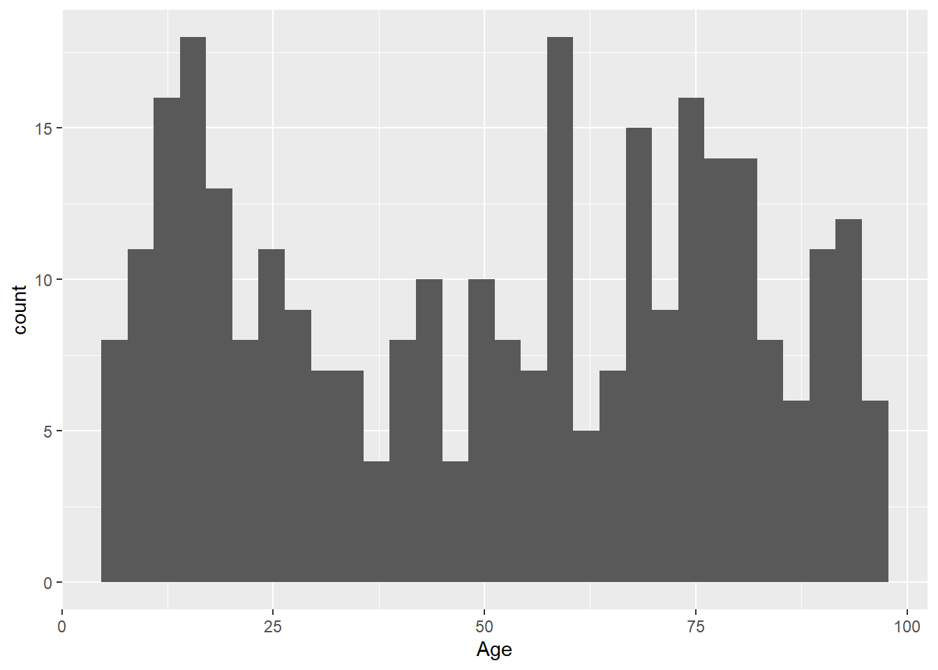

You don’t need to explicitly write the arguments:

ggplot(LOS_data, aes(x = Age)) +
  geom_histogram()

`stat_bin()` using `bins = 30`. Pick better value with `binwidth`.

Change the binwidth:

ggplot(data = LOS_data, mapping = aes(x = Age)) +
  geom_histogram(binwidth = 5)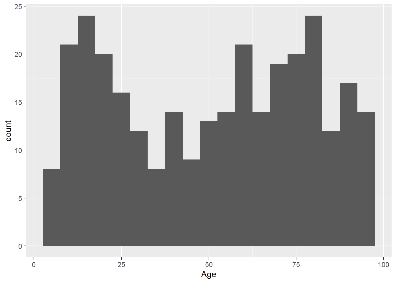

We want to subset the data to include only rows where the Organisation is equal to Trust1. We use the filter() function from the {dplyr} package to make a new data set:

library(dplyr)


Attaching package: 'dplyr'

The following objects are masked from 'package:stats':

    filter, lag

The following objects are masked from 'package:base':

    intersect, setdiff, setequal, union

LOS_trust1 <- LOS_data |>
  filter(Organisation == "Trust1")

Then use the same code to plot a histogram of age for only Trust 1 patient, but change the data we pass in:

ggplot(data = LOS_trust1, mapping = aes(x = Age)) +
  geom_histogram()

`stat_bin()` using `bins = 30`. Pick better value with `binwidth`.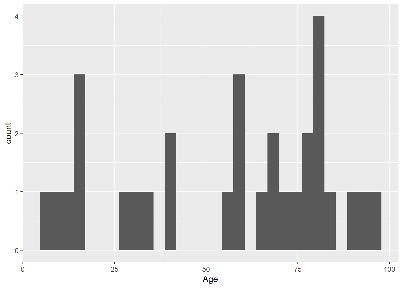

Example 4: Reading help files in R

See example

To read the help files for an R package or function, use a ? followed by the function name (with or without brackets). For example, to read the help files for the mutate() function in {dplyr}:

?mutate
?mutate()
help("mutate")

Example 5: Plotting multiple variables

See example

Do older patients stay longer?

ggplot(
  data = LOS_data,
  mapping = aes(x = Age, y = LOS)
) +
  geom_point()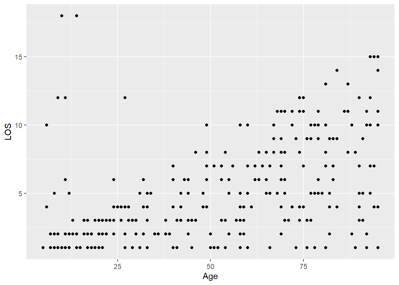

Does it vary by organisation? Let’s use colours to find out. R orders categories alphabetically unless you tell it otherwise, this is why Trust10 is before Trust2.

ggplot(
  data = LOS_data,
  mapping = aes(x = Age, y = LOS, colour = Organisation)
) +
  geom_point()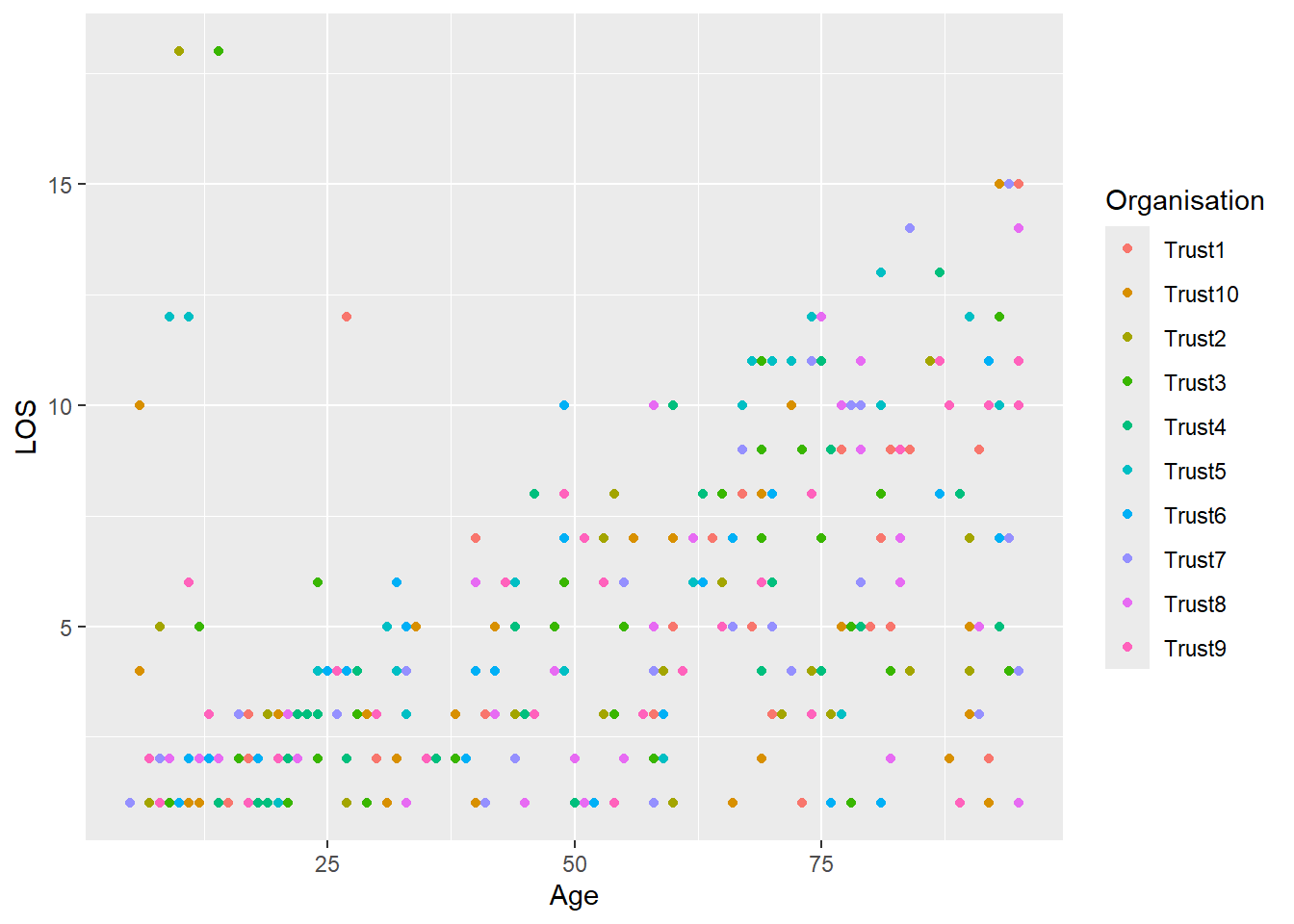

For colours based on numeric variables, R adds a continuous colour scale:

ggplot(
  data = LOS_data,
  mapping = aes(x = Age, y = LOS, colour = Age)
) +
  geom_point()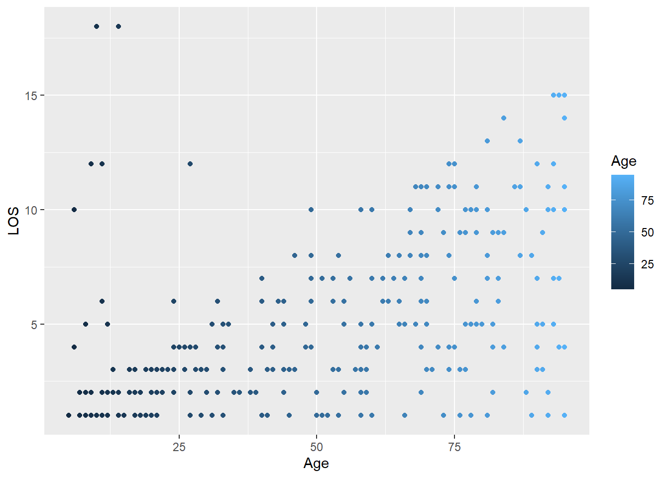

Sometimes we need to change the type of a variable for plotting e.g. from a numeric to a character.

ggplot(
  data = LOS_data,
  mapping = aes(x = Age, y = LOS, colour = Death)
) +
  geom_point()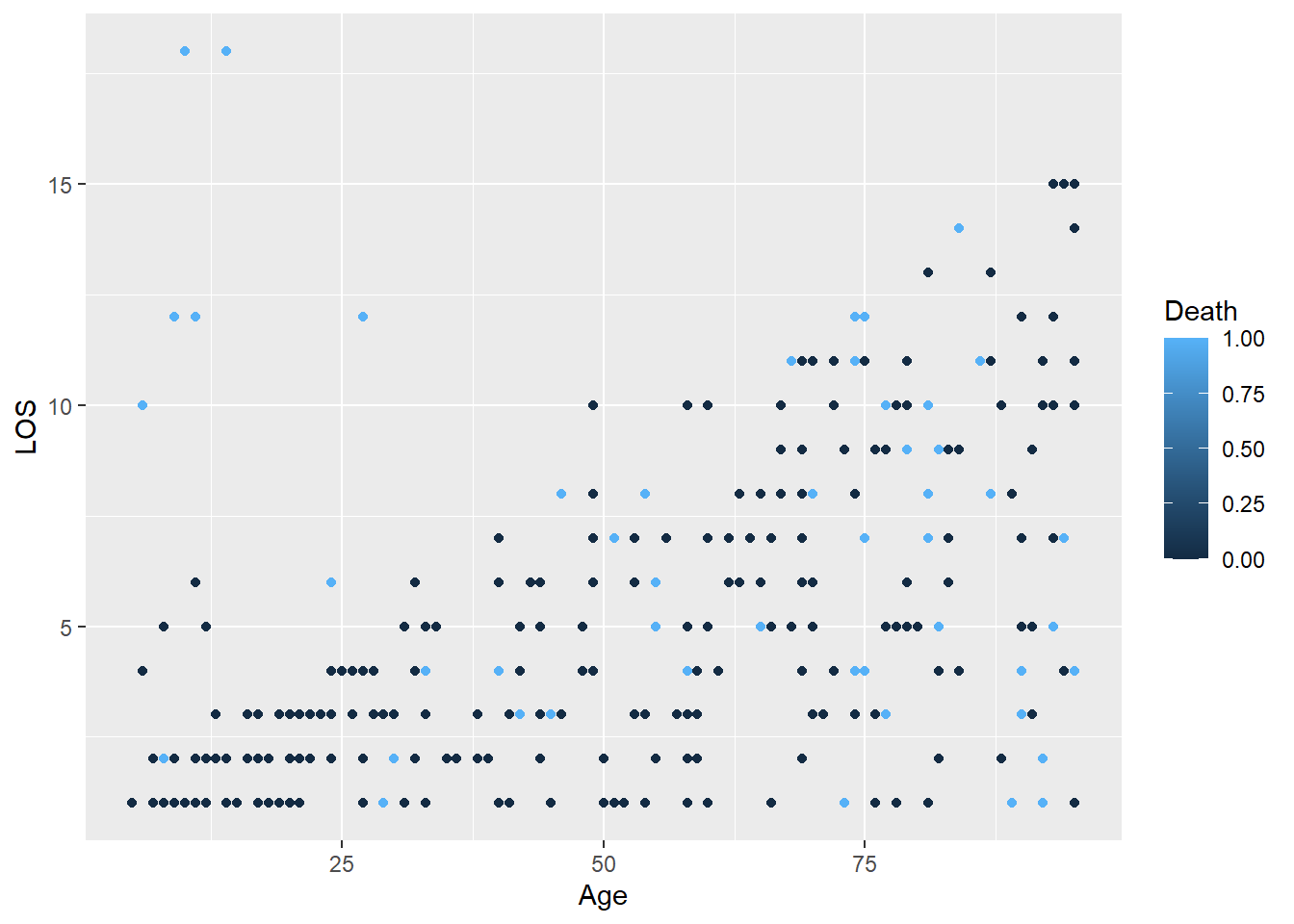

The Death column is encoded as 0 and 1 which R interprets as numbers, but these are actually categories (No and Yes). We can change it to a character or factor (ordered category).

ggplot(
  data = LOS_data,
  mapping = aes(x = Age, y = LOS, colour = factor(Death))
) +
  geom_point()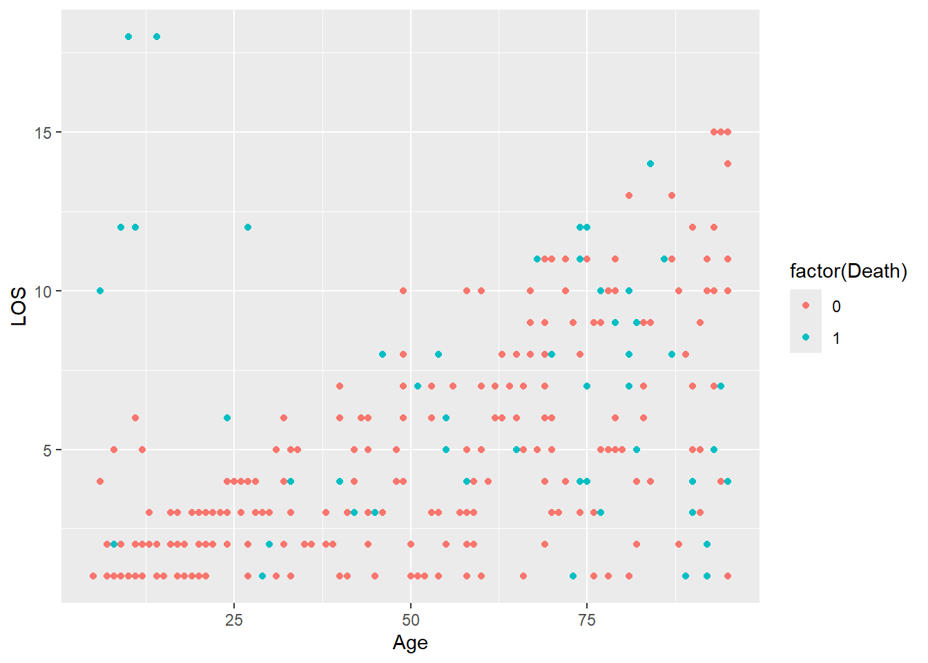

Example 6: Computing summary statistics

See example

What is the mean LOS?

In base R:

mean(LOS_data$LOS)

[1] 4.936667

LOS_data |>
  summarise(LOS_mean = mean(LOS))

# A tibble: 1 × 1
  LOS_mean
     <dbl>
1     4.94

Calculate the average LOS for each Organisation.

LOS_data |>
  group_by(Organisation) |>
  summarise(LOS_mean = mean(LOS))

# A tibble: 10 × 2
   Organisation LOS_mean
   <chr>           <dbl>
 1 Trust1           5.07
 2 Trust10          4.3 
 3 Trust2           4.23
 4 Trust3           5.07
 5 Trust4           4.87
 6 Trust5           6.1 
 7 Trust6           4.9 
 8 Trust7           5.1 
 9 Trust8           4.7 
10 Trust9           5.03

Also calculate the mean age for each Organisation:

LOS_data |>
  group_by(Organisation) |>
  summarise(
    LOS_mean = mean(LOS),
    Age_mean = mean(Age)
  )

# A tibble: 10 × 3
   Organisation LOS_mean Age_mean
   <chr>           <dbl>    <dbl>
 1 Trust1           5.07     55.4
 2 Trust10          4.3      51.0
 3 Trust2           4.23     51.2
 4 Trust3           5.07     47.9
 5 Trust4           4.87     49.5
 6 Trust5           6.1      45.7
 7 Trust6           4.9      48.6
 8 Trust7           5.1      53.7
 9 Trust8           4.7      51.4
10 Trust9           5.03     52.3

What about the standard deviation?

LOS_data |>
  group_by(Organisation) |>
  summarise(
    LOS_mean = mean(LOS),
    Age_mean = mean(Age),
    LOS_sd = sd(LOS),
    Age_sd = sd(Age)
  )

# A tibble: 10 × 5
   Organisation LOS_mean Age_mean LOS_sd Age_sd
   <chr>           <dbl>    <dbl>  <dbl>  <dbl>
 1 Trust1           5.07     55.4   3.52   28.2
 2 Trust10          4.3      51.0   3.35   29.5
 3 Trust2           4.23     51.2   3.51   27.3
 4 Trust3           5.07     47.9   3.98   28.4
 5 Trust4           4.87     49.5   3.42   26.4
 6 Trust5           6.1      45.7   4.30   28.3
 7 Trust6           4.9      48.6   3.34   27.8
 8 Trust7           5.1      53.7   3.82   29.2
 9 Trust8           4.7      51.4   3.71   27.8
10 Trust9           5.03     52.3   3.32   28.7

Example 7: Summary tables

See example

Drop the ID column, then make a summary table of the rest of the variables:

library(gtsummary)

Warning: package 'gtsummary' was built under R version 4.4.3

tbl1_data <- LOS_data |>
  select(-ID)
tbl1_data |>
  tbl_summary()

Characteristic	N = 300¹
Organisation
Trust1	30 (10%)
Trust10	30 (10%)
Trust2	30 (10%)
Trust3	30 (10%)
Trust4	30 (10%)
Trust5	30 (10%)
Trust6	30 (10%)
Trust7	30 (10%)
Trust8	30 (10%)
Trust9	30 (10%)
Age	54 (24, 76)
LOS	4.0 (2.0, 7.0)
Death	53 (18%)
¹ n (%); Median (Q1, Q3)

Group by Organisation:

tbl1 <- tbl1_data |>
  tbl_summary(by = Organisation)
tbl1

Characteristic	Trust1 N = 30¹	Trust10 N = 30¹	Trust2 N = 30¹	Trust3 N = 30¹	Trust4 N = 30¹	Trust5 N = 30¹	Trust6 N = 30¹	Trust7 N = 30¹	Trust8 N = 30¹	Trust9 N = 30¹
Age	62 (30, 80)	49 (26, 77)	57 (19, 74)	52 (21, 73)	48 (23, 75)	39 (18, 72)	49 (25, 74)	58 (26, 78)	51 (26, 79)	54 (26, 74)
LOS	5.0 (2.0, 7.0)	3.0 (2.0, 5.0)	3.0 (2.0, 6.0)	4.5 (2.0, 7.0)	4.0 (2.0, 8.0)	4.5 (2.0, 11.0)	4.0 (2.0, 7.0)	4.0 (2.0, 7.0)	3.0 (2.0, 7.0)	4.0 (2.0, 8.0)
Death	7 (23%)	4 (13%)	5 (17%)	6 (20%)	4 (13%)	7 (23%)	4 (13%)	8 (27%)	5 (17%)	3 (10%)
¹ Median (Q1, Q3); n (%)

Export to a Word document:

library(gt)
tbl1 |> 
  as_gt() |> 
  gtsave(filename = "Table 1.docx")

Example 8: Statistical tests

See example

Is the LOS significantly different for patients under the age of 50, compare to those who are 50 or older?

# Subset data
LOS_younger <- filter(LOS_data, Age < 50)
LOS_older <- filter(LOS_data, Age >= 50)

Are the means different?

t.test(LOS_younger$LOS, LOS_older$LOS)


    Welch Two Sample t-test

data:  LOS_younger$LOS and LOS_older$LOS
t = -8.0643, df = 296.03, p-value = 1.844e-14
alternative hypothesis: true difference in means is not equal to 0
95 percent confidence interval:
 -3.767660 -2.289483
sample estimates:
mean of x mean of y 
 3.321429  6.350000

Are the variances different?

var.test(LOS_younger$LOS, LOS_older$LOS)


    F test to compare two variances

data:  LOS_younger$LOS and LOS_older$LOS
F = 0.64874, num df = 139, denom df = 159, p-value = 0.009204
alternative hypothesis: true ratio of variances is not equal to 1
95 percent confidence interval:
 0.4704584 0.8977698
sample estimates:
ratio of variances 
         0.6487431