using Pkg
Pkg.add("PalmerPenguins")Introduction to Julia for R users
R
Julia
Quarto
This blog post will give R users an overview of what Julia is and why they might want to use it, introduce some data processing Julia packages, and show how they can incorporate Julia into existing R workflows.
If you’re an R user, you might be curious about trying another programming language. But you might also not be that enthusiastic about learning another language since it can be time-consuming, difficult, or tedious - especially if you already have code that works in R. This blog post aims to highlight some of the benefits that an R user might gain from using Julia - a high-level, general-purpose, open source programming language. It will also introduce some Julia packages that are based on packages built in R for an easier introduction to Julia, and show you how to interface between R and Julia.
Note
This blog post is a follow-up to Learning Julia with #TidyTuesday and Tidier.jl first published in June 2023. Though the first post is still a good introduction to plotting in Julia, some of the syntax may be outdated.
Why use Julia?
One of the main differences between Julia and R is that Julia is a compiled language, whereas R is an interpreted language (as is Python). Interpreted languages execute instructions directly line by line, i.e. translate code into machine language during execution. This is great for interactive debugging and user-friendliness but bad for speed.
Compiled languages, like Julia, convert code into machine language before running it, leading to faster execution. Since Julia compiles just in time (before code is executed), the user experience can be much like that of an interpreted language. This means you get the benefits of speed, but without losing the user-friendliness. The syntax of Julia is also simpler, with many built-in functions, compared to other compiled languages.
There are also some implementations in Julia that may not be available in R, or may not work well with large datasets or when models become too computationally expensive. Being able to work with both R and Julia gives you access to a wider range of tools - including approaches for Bayesian modelling, optimisation, symbolic modelling of systems, and solving differential equations.
Getting started with Julia
Let’s jump straight in to learning some Julia!
Installing Julia
There are a few different ways that Julia can be installed, depending on your operating system and how automated you want any updates to be in future. You can find the relevant links for your operating system at julialang.org/install. Make sure Julia is also added to your PATH so that other programmes can find it.
Note
You also need to decide where to run Julia code. You can run Julia code from a terminal, by typing Julia. However, much like running R code in a console isn’t the best way, I’d recommend using an IDE (integrated development environment). I’d recommend Positron or VSCode for Julia code. If you want to run Julia from RStudio, you may need to install JuliaCall first - see JuliaCall below.
You might want to read How to choose an IDE to help you decide!
Installing packages
Much like R (and other languages), Julia has an extensive collection of additional packages that can be installed. We’re going to need some data for our examples later on, so let’s install the PalmerPenguins package - you’re likely already familiar with the penguins dataset if you’re an R user!
First we need to install the package using:
Here, Pkg refers to Julia’s built-in package manager. The Pkg.add() command is a bit like the install.packages() function in R, so you only need to run it once.
TipStarting the Julia package manager
Typing ] also starts up the Julia package manager. You can then type add PalmerPenguins as an alternative way of installing packages. Either approach is fine.
We then load the PalmerPenguins package using:
using PalmerPenguinsThis is equivalent to library() in R and so needs to be run at the start of each session.
Loading data
Then we can use PalmerPenguins.load() to actually download the data file, and DataFrame() to convert it to a data frame.
using DataFrames
penguins = DataFrame(PalmerPenguins.load());
TipLoading from other sources
You won’t often be loading data straight from a package, instead you’re more likely to either connect to a database or load from an external file, such as a CSV. In Julia, the CSV.read() function from the CSV package provides functionality to read in data from a CSV file.
Tidier.jl
Tidier.jl is inspired by R’s tidyverse but developed specifically for Julia. Like the tidyverse package in R, it’s actually a collection of smaller packages - each for performing a specific set of tasks. In this blog post, we’ll focus on two of them:
- TidierData: for data wrangling and processing
- TidierPlots: for plotting data
Remember to install these packages using Pkg.add() first!
If you’re unfamiliar with
tidyversepackages or you’re just not a fan of them in R, I’d still encourage you to have a look atTidier.jl- but I’m not going to turn this into a base R versustidyversediscussion!
Data wrangling with TidierData.jl
Let’s perform some very simple data wrangling here, so you can see the comparison between dplyr in R, and TidierData.jl in Julia. Let’s filter the data to only look at complete rows, and to consider only female penguins. We’ll also convert the body mass from grams to kilograms, and drop the bill depth column since we won’t use it in later analysis.
Warning
The R examples use the penguins data from base R (available since version 4.5.0). It has slightly different column names to the version found in palmerpenguins, and to the Julia package.
The functions you’re likely familiar with from dplyr are named and work in the same way in TidierData.jl. For example, the filter() function lets you filter out rows of data based on some conditions, the mutate() function can be used to add or edit columns, and the select() function is used to choose a subset of columns to keep or drop.
using TidierData
penguins = @chain penguins begin
  @drop_missing()
  @filter(sex == "female")
  @mutate(body_mass_g = body_mass_g / 1000)
  @select(-bill_depth_mm)
end;library(dplyr)
library(tidyr)
penguins <- penguins |>
drop_na() |>
filter(sex == "female") |>
mutate(body_mass = body_mass / 1000) |>
select(-bill_dep)There are a couple of syntax differences to be aware of:
- In R, we use the pipe operator (either
|>or%>%) in between functions to chain functions together. In Julia, we use the@chainmacro instead and every function betweenbeginandendmodifies the data mentioned at the beginning. - In Julia, some functions are pre-fixed with
@because they use macros to simplify the syntax.
TipSuppressing output
You’ll notice that some lines of code in Julia have a ; at the end of them. This suppresses the output i.e. stops the dataset from printing in the console or in a script. You can also use ; if you want to define multiple variables on the same line.
Plotting with TidierPlots.jl
TidierPlots.jl is a 100% Julia implementation of the R package ggplot2 powered by Makie.jl. Below, we’ll compare the code and outputs for two different types of plots: a simple boxplot, and a scatter plot with some custom styling.
Let’s start with a simple boxplot of flipper lengths across the three species of penguins.
using TidierPlots
ggplot(penguins, @aes(x = species, y = flipper_length_mm)) +
  geom_boxplot(@aes(fill = species))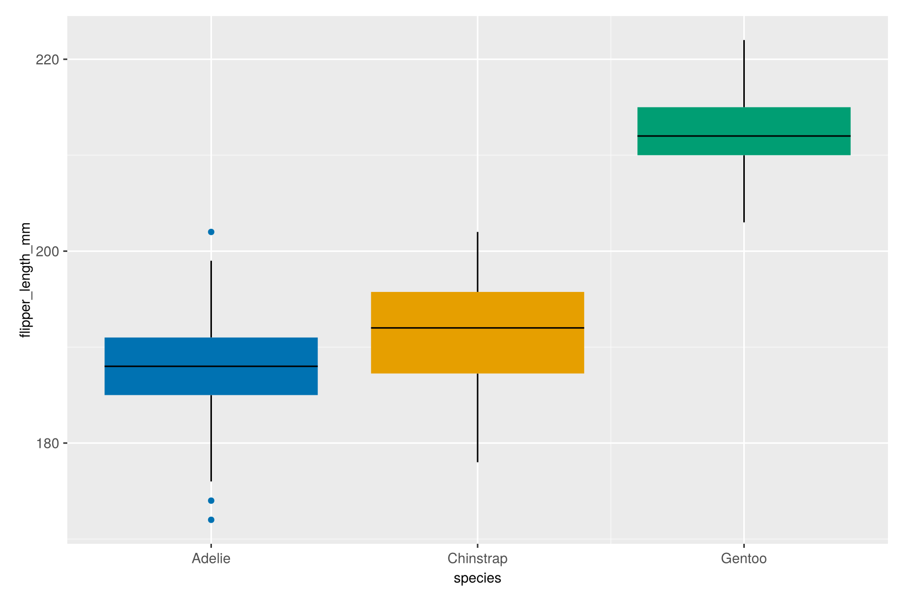
library(ggplot2)
ggplot(penguins, aes(x = species, y = flipper_len)) +
  geom_boxplot(aes(fill = species))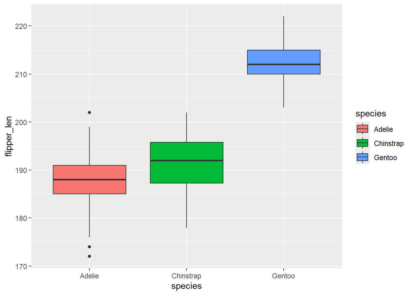
If you toggle between the Julia and R versions, you’ll see that the code is almost identical. In fact, for this simple example, there are only two differences:
- The way that the packages are loaded with either
usingin Julia orlibrary()in R as we’ve already discussed. - The pre-fixing of the
aes()function in Julia with@, which again we’ve already discussed in the data wrangling section.
You’ll also notice a couple of differences in the output:
- The default colour scheme is different. The Julia version uses a slightly more accessible colour palette - and I have to admit, I do prefer it to the
ggplot2colours! - You’ll also notice there is no legend added by default which, in this example, is again a better design since the x-axis labels effectively act as a legend.
Otherwise, the outputs are very similar - including that grey background!
It’s easy to compare code for such a simple plot and say they look similar, but what happens when we want to add a lot of custom styling to make our plots look nicer? Is it still that similar? Let’s create a scatter plot of flipper length and bill length, again coloured by species. This time, we’ll also use our own colours for each species, apply a different theme with some specific tweaks, and add some text.
ggplot(penguins, @aes(x = flipper_length_mm, y = bill_length_mm)) +
  geom_point(@aes(color = species, shape = species), size = 14) +
  scale_shape() +
  scale_color_manual(values = ["darkorange", "purple", "cyan4"]) +
  labs(title = "Flipper and bill length",
       subtitle = "Measurements for Adelie, Chinstrap and Gentoo penguins",
       x = "Flipper length (mm)",
       y = "Bill length (mm)",
       color = "Penguin species",
       marker = "Penguin species") +
  theme_minimal()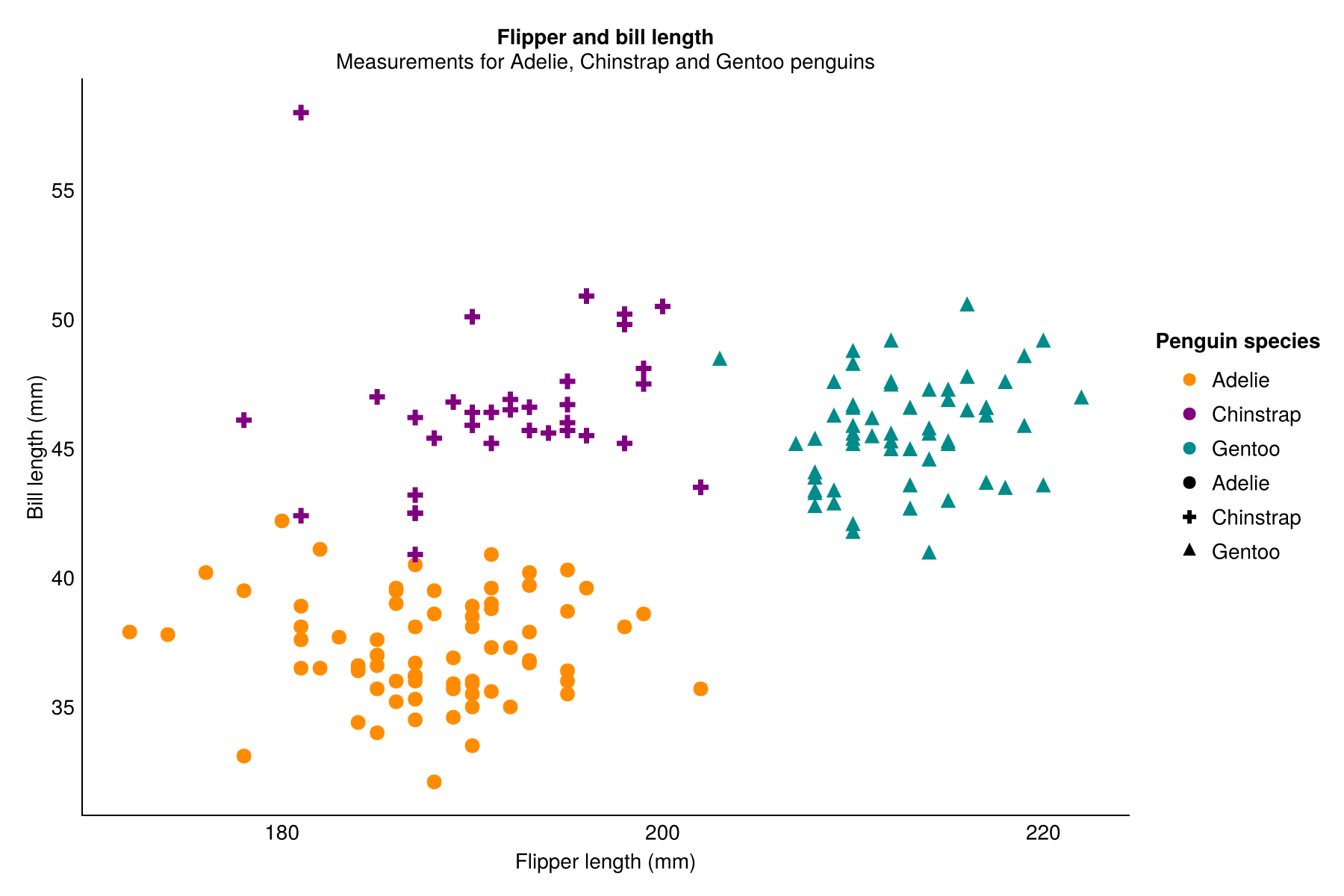
ggplot(penguins, aes(x = flipper_len, y = bill_len)) +
  geom_point(aes(color = species, shape = species), size = 3) +
  scale_color_manual(values = c("darkorange", "purple", "cyan4")) +
  labs(
    title = "Flipper and bill length",
    subtitle = "Measurements for Adelie, Chinstrap and Gentoo penguins",
    x = "Flipper length (mm)",
    y = "Bill length (mm)",
    color = "Penguin species",
    shape = "Penguin species"
  ) +
  theme_minimal()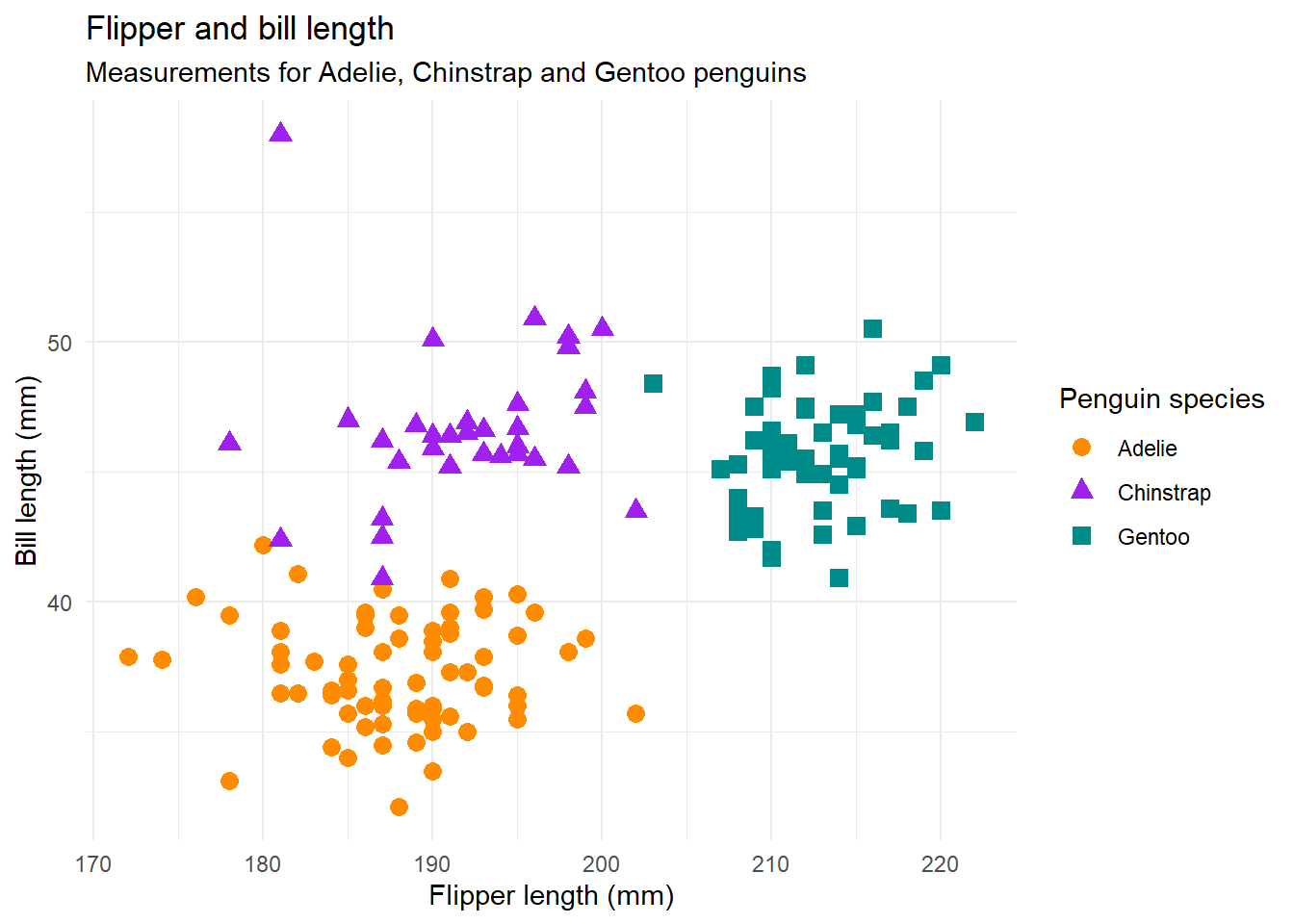
Again, there are some differences in both the code and the output - partly due to current limitations in TidierPlots.jl.
- The
theme_minimal()function produces a slightly different theme from the version inggplot2- it’s a bit more liketheme_classic()in {ggplot2}. - The title and subtitle are centre aligned instead of aligned to the left hand side of the panel.
- The default markers are different shapes with a slightly smaller default size. In Julia, we also need to add
scale_shape()to make this work, whereas R does it by itself. Confusingly in Julia, thelabs()argument to edit the shape legend title is calledmarkerinstead ofshape, even though other elements useshape. - The legends also don’t quite properly combine - instead the shape and colour items are listed twice - but legends in
TidierPlots.jlare still a work in progress!
Note
You can view some of the other visualisations I’ve created using Julia (with code) in the Quarto document published at nrennie.quarto.pub/juliatuesday. You can also view the source code on GitHub, though again it might be a little outdated in terms of syntax.
Overall, TidierPlots.jl isn’t quite as powerful as ggplot2 yet, but if you’re creating fairly simple plots you should be able to do what you need. Many of the default settings for the Julia implementations result in nicer looking plots so you may actually need to make fewer tweaks!
Combining R and Julia
Although Tidier.jl is an easy way for tidyverse R users to get started with Julia, I’m not suggesting you re-write every single piece of R code you have in Julia. Instead, I’d recommend finding the bottlenecks in your code (the bits that are slow) and converting those to Julia - make code changes only where the difference in speed really matters!
So how do we interface R and Julia?
JuliaCall
JuliaCall is an R package that allows you to run Julia code from R. JuliaCall isn’t the only R package that provides an interface with Julia but it is the one used by Quarto (which we’ll discuss more later) so we’ll focus on it here.
Start by installing and loading the package as you normally would:
library(JuliaCall)If you don’t already have Julia installed, you can run:
install_julia()This installs Julia for you, makes sure it’s in the right place, and that R can find it. At the start of each new R session, you should also run:
julia <- julia_setup()You can then evaluate Julia code in R using the julia_eval() function. For example, to calculate the square root of 2 (where the calculation is performed in Julia), we do:
julia_eval("sqrt(2)")[1] 1.414214Note that both julia_eval("sqrt")(2) and julia_call("sqrt", 2) are alternative ways of running julia_eval("sqrt(2)"). This can be really useful if you want to pass a value you’ve calculated in R in as an argument to a Julia function. You can save the result of the computation from Julia in the normal way:
y <- julia_eval("sqrt(2)")and then use it in R calculations as you normally would:
y^2[1] 2
TipRunning Julia scripts in R
Writing and running Julia code in the form of a character string is not a great experience for longer pieces of code due to the lack of syntax highlighting and formatting. Instead, you’re more likely to write your Julia code in a separate .jl script. You can run the whole script in R using julia_source():
julia_source("script.jl")If we want to go the opposite way and use values that we have calculated in R within our Julia code, we can pass an object from R to Julia using julia_assign(). The following code calculates the exponential of 5 in R, and assigns it to a variable a which exists in R. The julia_assign() passes that value to Julia (converting the type correctly) and assigns it to the variable x which exists in Julia.
a <- exp(5)
julia_assign("x", a)
We can check it works by evaluating x in Julia using julia_eval() in R:
julia_eval("x")[1] 148.4132
Tip
RCall
RCall allows you to call R from Julia. It’s very similar to JuliaCall, but the languages are the other way around.
Quarto
Quarto is an open-source scientific and technical publishing system that lets you create dynamic documents, presentations, websites, and books by integrating markdown with code to produce reproducible outputs. It has native support for multiple languages including both R and Julia. And that makes is one of the easiest ways to combine them.
There are several options for running both Julia and R code in the one document:
- Use the
knitrengine, and theJuliaCallR package will run your Julia code in much the same way we’ve discussed in this blog post already. - Use the
juliaengine, which usesQuartoNotebookRunner.jlalongside theRCallJulia package to render the document.
By default, Quarto sets the engine based on which language is used first in the document. However, I’d recommend specifying a different one if the first code block isn’t the most used language in the document. Technically, you can also use the jupyter engine but I’d probably stick to either julia orknitr unless you’re also including Python code. If you’re an R user, you’re likely already familiar with the knitr engine for Quarto or R Markdown documents so it might be the best first choice.
As a short example of how to combine the two using a knitr engine, here’s a little template:
---
title: "My Julia + R Document"
engine: knitr
---

```{julia}
x = 7 + 9
```

```{r}
plot(1:10, 1:10)
```
It is really is as simple as writing R and Julia code blocks. If you want to pass objects between code blocks, rather than just evaluating them separately, you can use some of the approaches we’ve already discussed from JuliaCall.
Further resources
If you’re thinking about working with Julia as an R user, these are some further resources you might find helpful:
Julia documentation: docs.julialang.org
Tidier.jldocumentation: tidierorg.github.io/Tidier.jlTidier.jlblog post about why R users should consider usingTidier.jl: tidierorg.github.io/Tidier.jl/Why-should-I-consider-using-Tidier.jl?Thread by Karandeep Singh on the process of moving from Julia to R: www.upcarta.com/resources/some-r-julia-tips
Documentation on how to integrate R with JuliaHub: info.juliahub.com/resources/integrating-r-with-juliahub
ImportantConference session
I’ll be talking about this topic at the Royal Statistical Society International Conference in Edinburgh on September 2, 2025.
Slides can be found here: nrennie.rbind.io/talks/rss-intro-julia
Reuse
Citation
BibTeX citation:
@online{rennie2025,
  author = {Rennie, Nicola},
  title = {Introduction to {Julia} for {R} Users},
  date = {2025-08-18},
  url = {https://nrennie.rbind.io/blog/introduction-julia-r-users/},
  langid = {en}
}
For attribution, please cite this work as:
Rennie, Nicola. 2025. “Introduction to Julia for R Users.”
August 18. https://nrennie.rbind.io/blog/introduction-julia-r-users/.