Engaging and effective data visualisations

24 March 2026

Dr Nicola Rennie

Who am I?

Data visualisation specialist, mainly working with R, Python, and D3.js.

Background in statistics, operational research, and data science consultancy.

Co-author of Royal Statistical Society’s Best Practices for Data Visualisation guidance.

How did I get here?

• 2014-2017: Undergraduate in maths
• 2017-2021: STOR-i
  • Thesis: Detecting demand outliers in transport systems
  • Chapter on Analysing and visualising bike sharing demand with outliers
• 2021-2023: Data science consultancy
• 2023-2025: Back to academia as a Lecturer in Health Data Science
• 2025-Present: Data visualisation specialist at ONS

How did I get into data visualisation?

• 2021: Started making and posting data visualisation on social media; writing blog posts; delivering more talks
• 2022: Making dashboards is part of my job
• 2023-2024: Co-authored the Royal Statistical Society’s Best Practices for Data Visualisation guidance
• 2024-2025: Book contract to write about visualisation in R
• 2025-Present: Data visualisation is my full time job

What’s this session about?

In this session we will cover…

• why you should visualise data;

• choosing a chart type;

• some guidelines for making better charts;

• examples of good and bad charts!

The role of visualisation

Why visualise data?

Data visualisation has two main purposes:

• Exploratory: informs data analysis
• Explanatory: communicating insights and results

Exploratory data visualisation

What does this data look like?

Statistic	Value
Mean(x)	54.26
Mean(y)	47.83
Standard deviation(x)	16.77
Standard deviation(y)	26.94
Correlation(x, y)	-0.06

Summary statistics aren’t enough!

Explanatory data visualisation

Communicating insights with data visualisation

Grab attention

Visualisations stand out. If a reader is short on time or uncertain about whether a document is of interest, an attention-grabbing visualisation may entice them to start reading.

Improve access to information

Textual descriptions can be lengthy and hard to read, and are frequently less precise than a visual depiction showing data points and axes.

Summarise content

Visual displays allow for summarising complex textual content, aiding the reader in memorising key points.

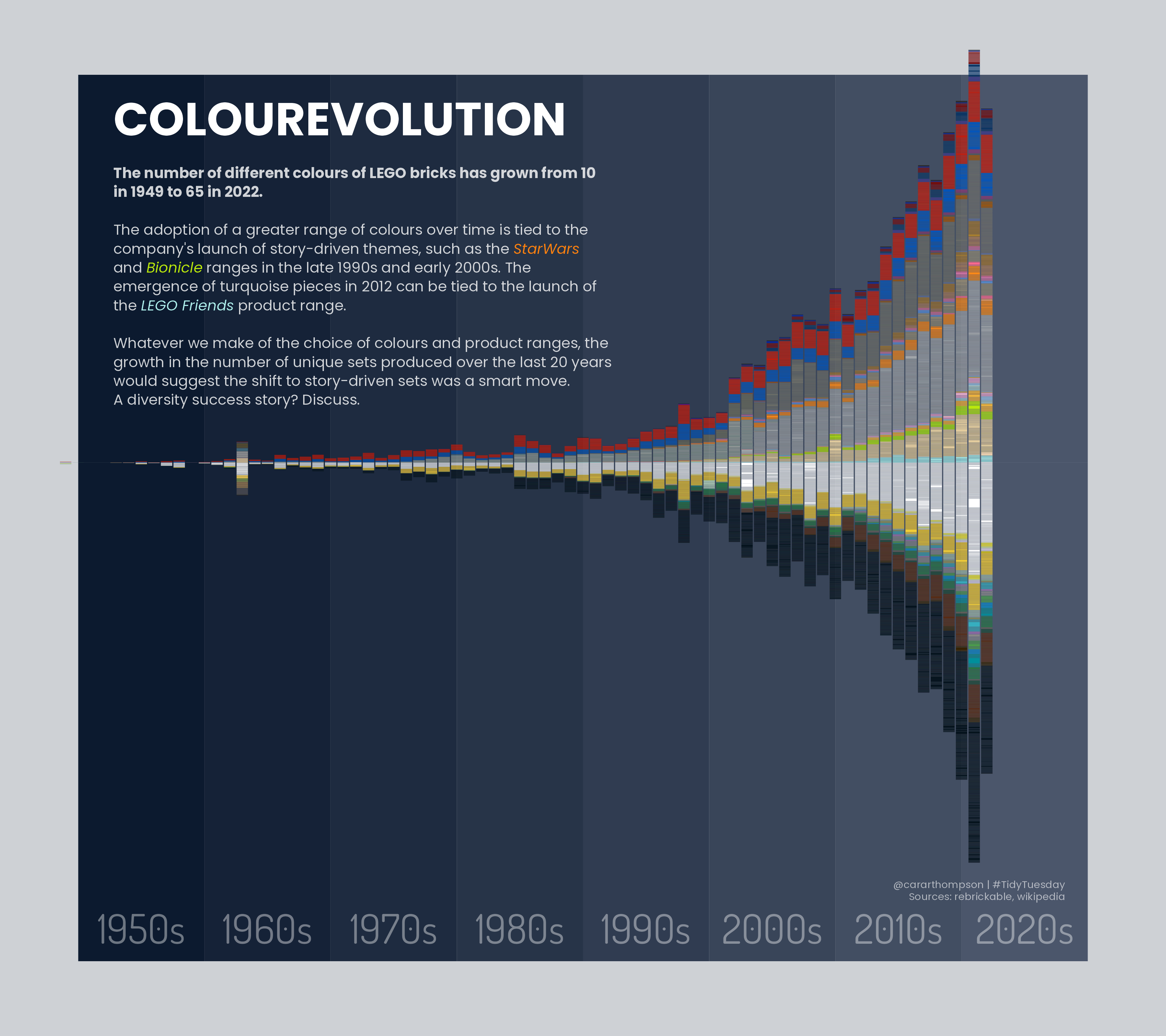
Communicating insights with data visualisation

John Snow collected data on cholera deaths and created a visualisation where the number of deaths was represented by the height of a bar at the corresponding address in London.

This visualisation showed that the deaths clustered around Broad Street, which helped illustrate the cause of the cholera transmission, the Broad Street water pump.

Snow. 1854.

Choosing a chart type

What’s the purpose of your visualistion?

Data visualisations must serve a purpose.

Ask yourself:

• What is the purpose?
• Does the visualisation support the purpose?
• Is it quick, accurate, and intuitive?

What are you trying to communicate?

Detailed, accurate numbers?

Or the big picture message?

Common relationships

• Correlation: The relationship between two variables.

• Deviation: The difference between a value and an average or another value.

• Distribution: How data values are spread for a variable.

• Geography: The pattern of data across different locations or areas.

• Magnitude: The size of values.

• Parts of a whole: The relative sizes of components within a whole.

• Ranking: The position of data within a hierarchy or scale.

• Time: How a value changes over time.

Visual vocabulary

It’s not just about the type of data…

Does the chart type match the purpose?

Why do pie charts have a bad reputation?

Why do 3D charts have a bad reputation?

What value does the bar represent?

It’s not that 3D charts are always bad!

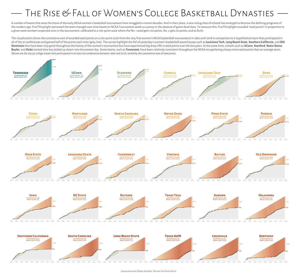
Avoid spaghetti plots!

Effectively plotting multiple values

Alternatives to spaghetti:

• Show a smaller number of lines (e.g. compare a few countries to average)
• Use colour only to highlight lines
• Use facets (AKA small multiples)

Small mutliples allow clearer comparison

Plotting variables on different scales

Effectively plotting on different scales

Some alternatives:

• Separate plots, each with their own axis, and place the plots side-by-side.
• Plot different variables on the x- and y- axis.
• Rescale the variables, rather than the axis.

Comparing distributions

Small multiples improve clarity

Arrange for comparison

Axes

Longer labels are best on the y-axis, horizontally.

How do the two bars compare?

Axes don’t always have to start at zero

Order categories…

…in a sensible way

Source: Georgia Department of Public Health

Order categories appropriately

Default:

Magnitude ordered:

Naturally ordered:

Activity 1

In groups, discuss the following chart. What is good and bad about it?

Source: commonslibrary.parliament.uk/general-election-2019-how-many-women-were-elected available under Open Parliament Licence.

Break

Styling charts

Colours

Why use colours in data visualisation?

• Colours should serve a purpose, e.g. discerning groups of data

• Colours can highlight or emphasise parts of your data.

• Not always the most effective for, e.g. communicating differences between variables.

Types of colour palette

Different types of colour palettes…

… for different types of data.

Is this a good choice of colours?

Consider accessibility

Do symbols or patterns help?

Use intuitive colours where appropriate

Example: red and blue used to show hot and cold

Tip: never switch to the opposite meaning!

Are intuitive colours always best?

Example: pink and blue used to show women and men

Tip: think about colour associations.

Don’t reinforce negative stereotypes

“7 out of 8 female readers might not be particularly appreciative of [being represented by pink].”

Source: visualisingdata.com

Choosing good colours

• Okabe-Ito palette

• Paul Tol’s palettes

• ColorBrewer

Don’t rely on colour

• Use direct labels over a legend if you can
• Use shapes and patterns and/or small multiples
• If you have to use a legend, it should follow the order of the data

Fonts

Choose clear fonts

• Font size: larger fonts are (usually) better

• Font colour: ensure sufficient contrast

• Font face: highlight text using bold font, avoid italics

Tip: Check the contrast of the text colour against the background colour with webaim.org/resources/contrastchecker

Consider associations of fonts

Font family:

• choose a clear font
• with distinguishable features
• pick something familiar
• consider associations

Text

Use annotations to add context

• Give context, such as thresholds or important dates.
• Highlight what a user should look at.
• Keep annotations concise and close to the part of the chart they relate to.

Tip: If there’s something specific you want someone to look at, a big arrow pointing at it helps.

Use narrative titles to summarise

• Describe the main trend you want the chart to show to the user.
• Users are more likely to understand and remember the main trend from a chart where it is also in the chart title.
• If the trend described in your chart title is not the most prominent visual trend in the chart, consider what and how you are visualising.

Change in temporary accommodation over time

The number of households, and households with children, in temporary accommodation in Scotland are at record highs

Interactive charts

Types of interactive charts

• Passive interaction e.g. tooltips, crosshairs on hover, animations
• Explorer tools with user inputs e.g. drop down menu
• Scrollytelling

Just because you can, doesn’t mean you should.

Complex charts need explanation

Activity 2

Here’s a chart. You have 10 minutes to improve it as much as you can.

Activity 2: Python

import plotnine as gg
from palmerpenguins import load_penguins

Hints:

• Try scale_fill_manual() to change the colours
• Try coord_flip() to place category names on y-axis
• Try labs() to add some text

Activity 2: R

Hints:

• Try scale_fill_manual() to change the colours
• Try coord_flip() to place category names on y-axis
• Try labs() to add some text

Default chart

ggplot(
  data = penguins,
  mapping = aes(x = species, y = body_mass, fill = sex)
) +
  geom_boxplot()

Change the chart type

g <- penguins |>
  tidyr::drop_na(sex) |>
  ggplot(
    mapping = aes(x = body_mass, fill = sex)
  ) +
  geom_density(alpha = 0.5) +
  facet_wrap(~species, ncol = 1)
g

Improve colours

g <- g +
  scale_fill_manual(
    values = c("#653FA2", "#119DA4")
  )
g

Improve text

g <- g +
  labs(
    title = "Male penguins have higher body mass than females of the same species",
    subtitle = "Body mass (g)",
    caption = "Source: palmerpenguins",
    x = "Body mass (g)",
    y = NULL,
    fill = NULL
  )
g

Improve theme

library(ggtext)
g <- g +
  theme_minimal(base_size = 15) +
  theme(
    legend.position = "top",
    # Clean up y axis
    axis.text.y = element_blank(),
    axis.ticks.y = element_blank(),
    panel.grid.major.y = element_blank(),
    # Wrap, embolden title
    plot.title = element_textbox_simple(
      face = "bold"
    ),
    strip.text = element_text(
      face = "bold",
      hjust = 0
    )
  )
g

Before and after

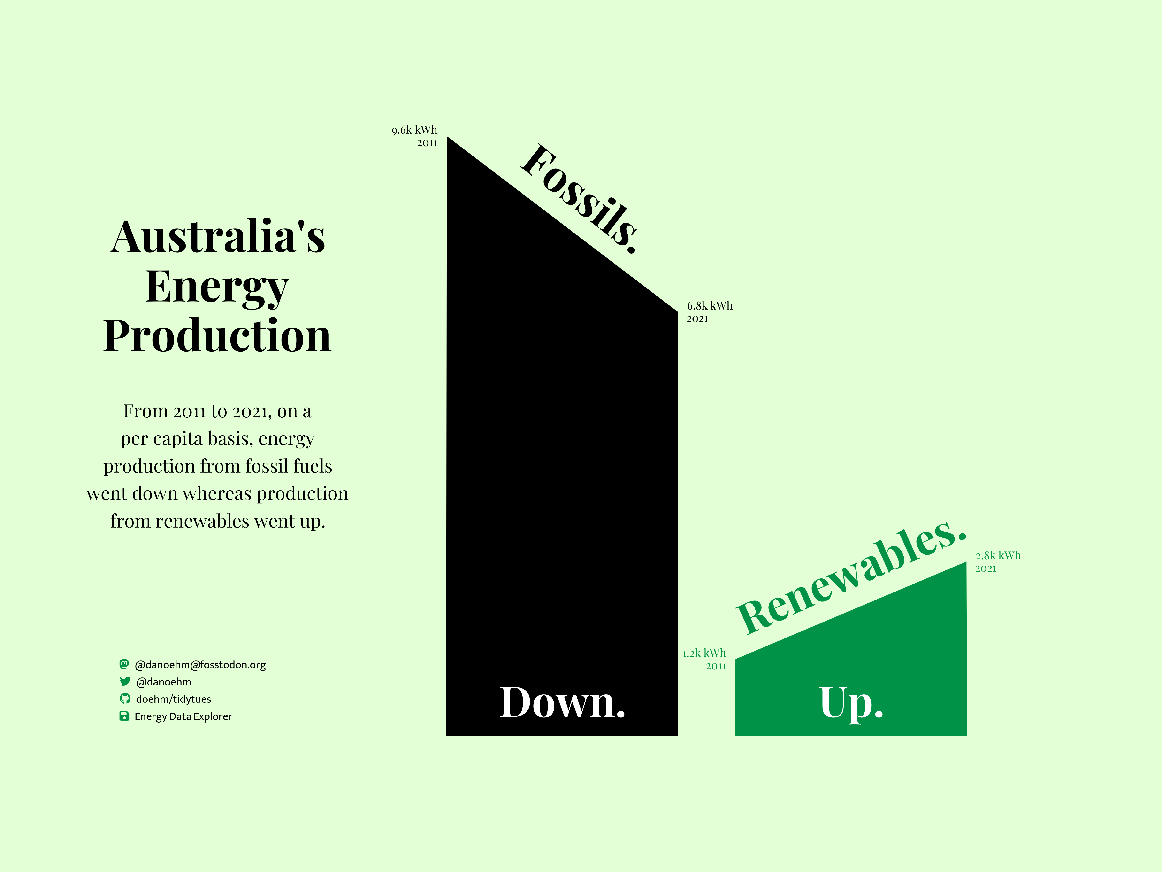
Good charts don’t have to be boring!

Cara Thompson (cararthompson.com)

Cedric Scherer (cedricscherer.com)

Good charts don’t have to be boring!

Tanya Shapiro

Dan Oehm (gradientdescending.com)

If you want to design better data visualisations…

• Know your audience
• Know your message
• Design charts to communicate your message to your audience

Resources

• ONS Data Visualisation Guidance: service-manual.ons.gov.uk/data-visualisation

• RSS Best Practices for Data Visualisation Guidance: rss.org.uk/datavisguide

• Data Visualisation Resources: nrennie.rbind.io/data-viz-resources

• The Art of Data Visualization with ggplot2: nrennie.rbind.io/art-of-viz

Slides: nrennie.rbind.io/stori-spring-school-2026

Questions?

nicola-rennie nrennie nrennie nrennie.rbind.io