Examples

Set up

Load packages:

library(dplyr)
library(ggplot2)
library(ggtext)
library(ggview)
library(glue)
library(showtext)
library(tidyr)
library(tidytuesdayR)

Load data using the tidytuesdayR package:

tuesdata <- tt_load("2023-01-31")
cats_uk <- tuesdata$cats_uk
cats_uk_reference <- tuesdata$cats_uk_reference

Exploratory work

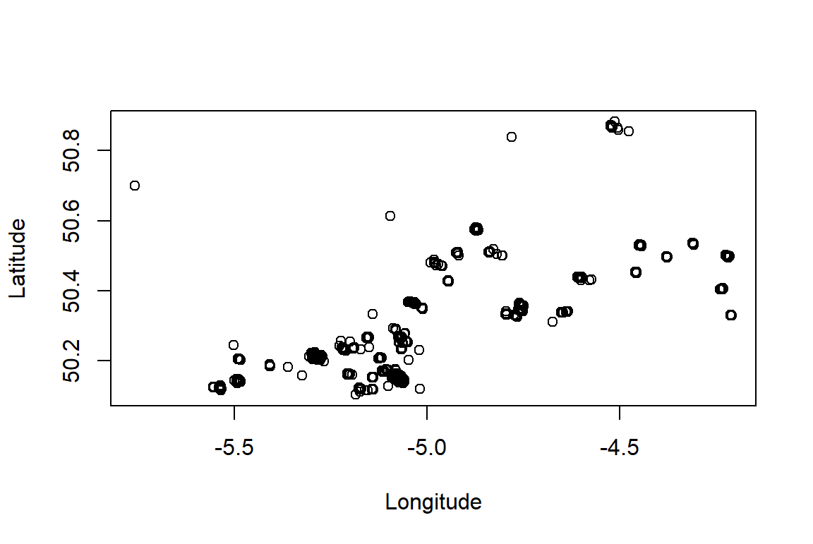
plot(
  x = cats_uk$location_long,
  y = cats_uk$location_lat,
  xlab = "Longitude",
  ylab = "Latitude"
)

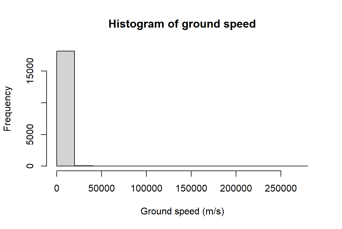
hist(
  x = cats_uk$ground_speed,
  xlab = "Ground speed (m/s)",
  main = "Histogram of ground speed"
)

barplot(table(cats_uk_reference$hrs_indoors))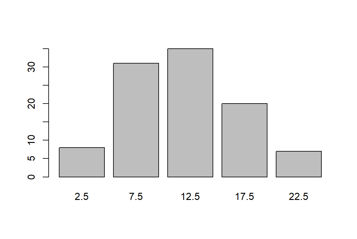

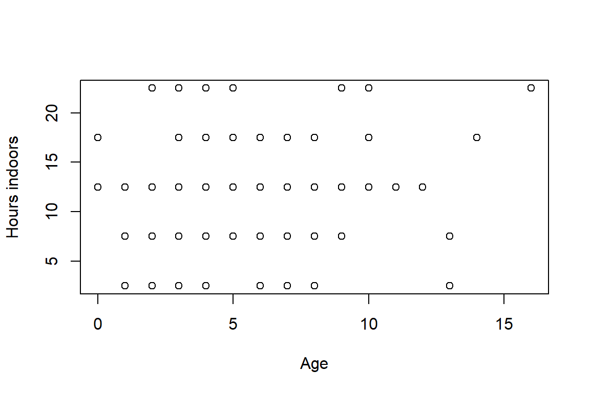
plot(
  x = cats_uk_reference$age_years,
  y = cats_uk_reference$hrs_indoors,
  xlab = "Age",
  ylab = "Hours indoors"
)

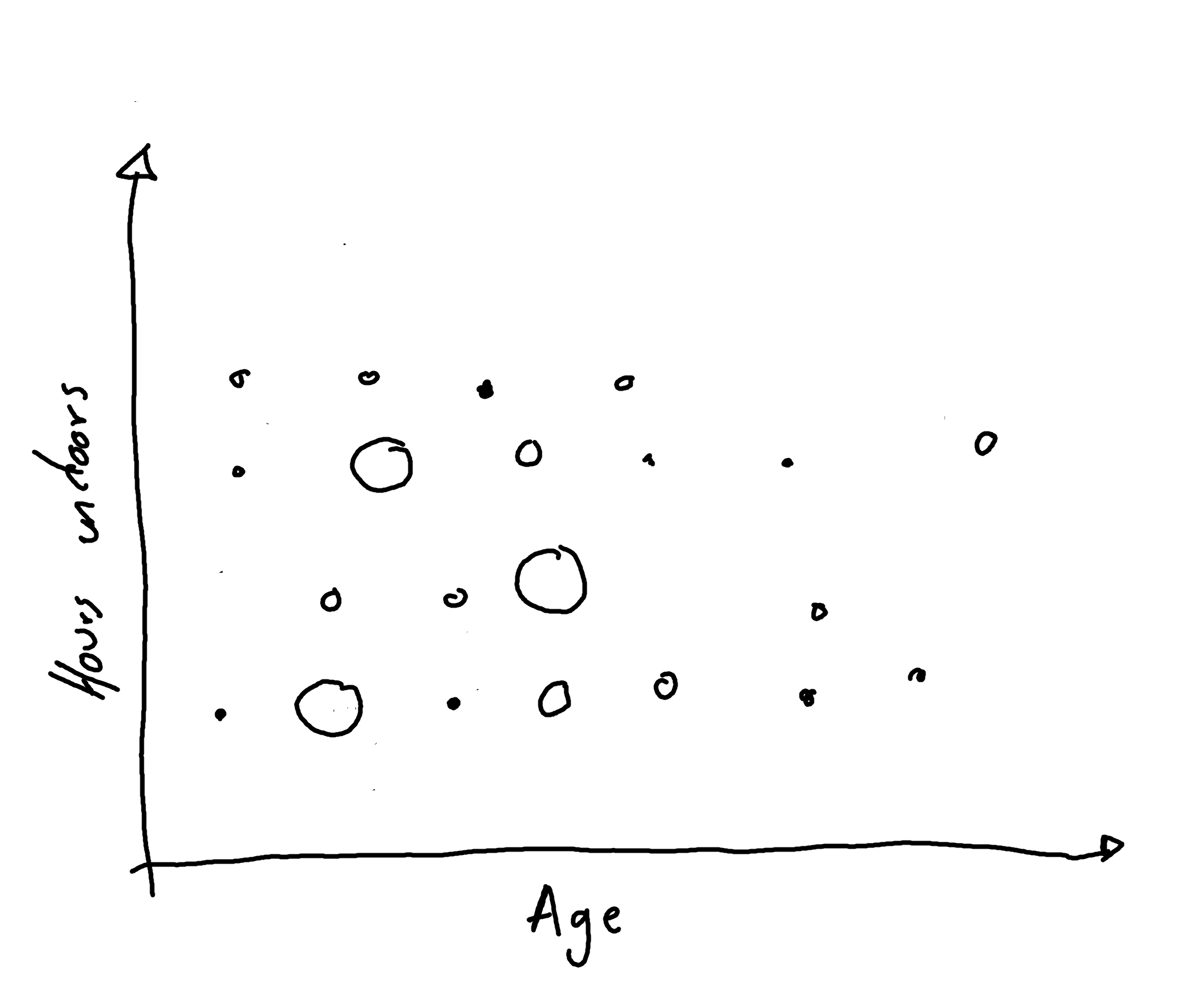
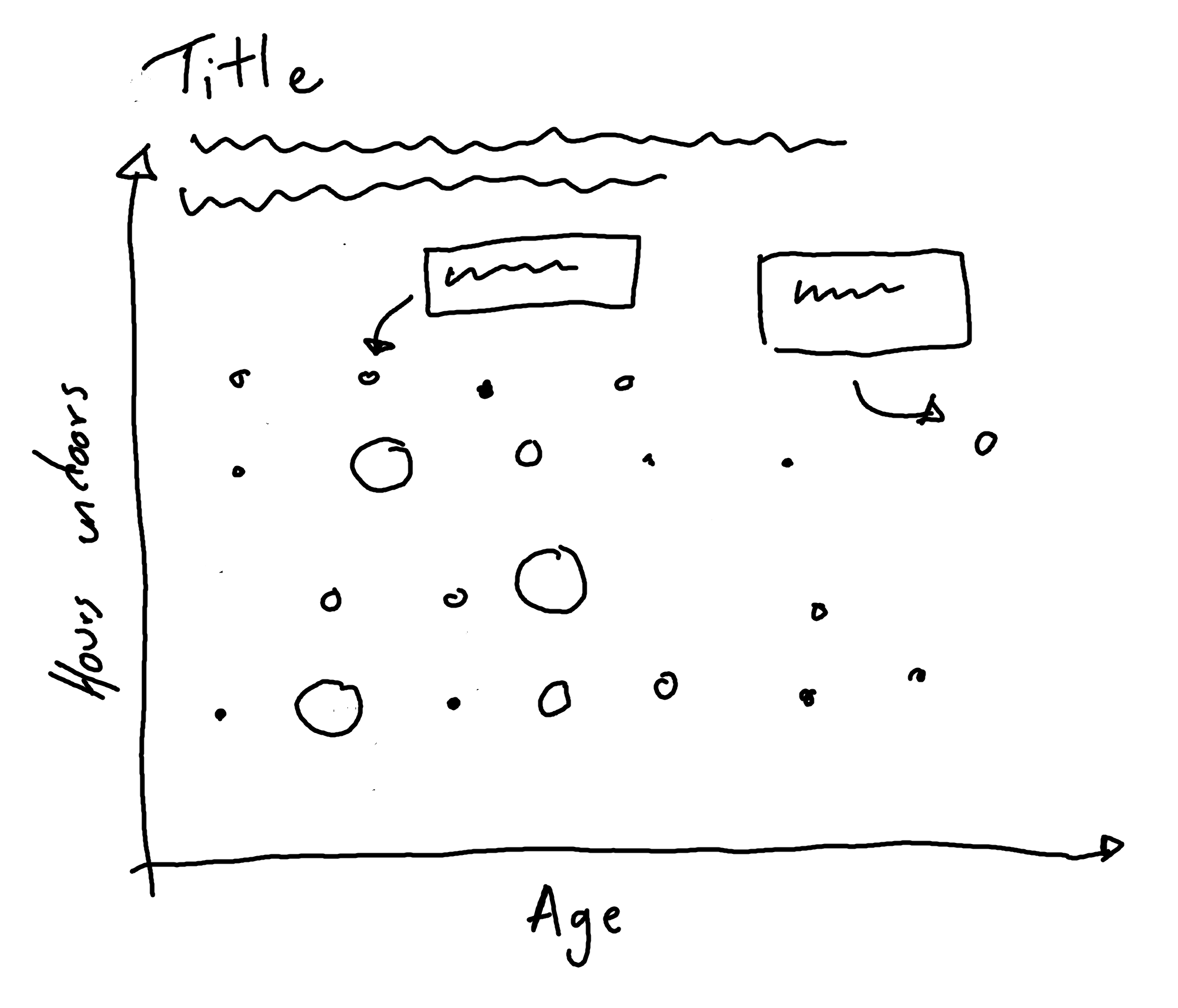
Sketching ideas

Initial draft

plot_data <- cats_uk_reference |>
  select(age_years, hrs_indoors) |>
  mutate(hrs_indoors = factor(hrs_indoors)) |>
  count(age_years, hrs_indoors) |>
  drop_na()

basic_plot <- ggplot(
  data = plot_data,
  mapping = aes(
    x = age_years,
    y = hrs_indoors,
    size = n
  )
) +
  geom_point()
basic_plot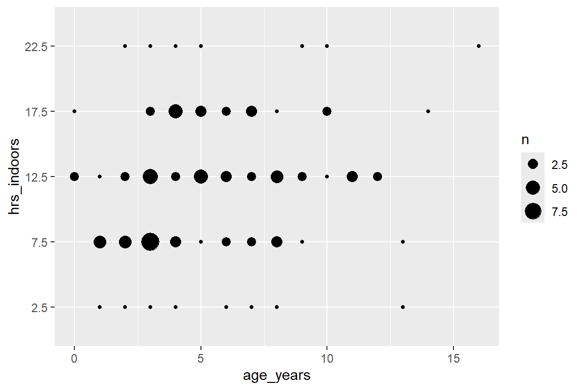

Use ggview to preview your plots at the desired size and resolution by adding the following to the end of your ggplot2 call (interactively in RStudio):

basic_plot +
  canvas(
    width = 5, height = 7,
    units = "in", bg = "white",
    dpi = 300
  )

Advanced styling

Colours and fonts

text_col <- "#152826"
highlight_col <- "#914D76"
bg_col <- "white"

basic_plot <- ggplot(
  data = plot_data,
  mapping = aes(
    x = age_years,
    y = hrs_indoors,
    size = n
  )
) +
  geom_point(color = highlight_col) +
  scale_size(breaks = c(3, 6, 9))
basic_plot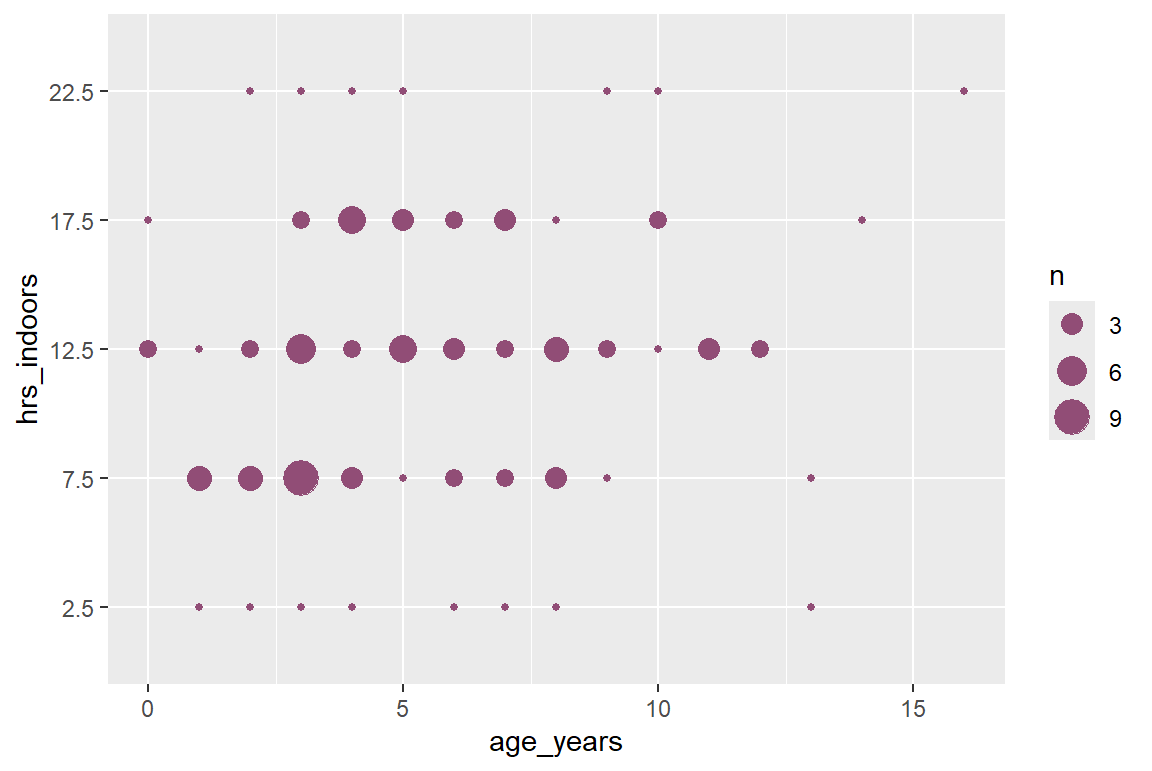

font_add_google(name = "Chewy")
font_add_google(name = "Ubuntu")
showtext_auto()
showtext_opts(dpi = 300)
title_font <- "Chewy"
body_font <- "Ubuntu"

Annotations and text

annot_oldest <- cats_uk_reference |>
  slice_max(age_years) |> 
  mutate(label = glue("The oldest cat is {animal_id} who is {age_years} years old.")) |> 
  select(hrs_indoors, age_years, label)

annotated_plot <- basic_plot +
  geom_textbox(
    data = annot_oldest,
    mapping = aes(
      x = age_years - 2.5,
      y = factor(hrs_indoors),
      label = label
    ),
    halign = 0.5,
    hjust = 0.5,
    size = 2.5,
    lineheight = 0.5,
    family = body_font,
    box.color = text_col,
    color = text_col,
    maxwidth = unit(1, "in")
  )
annotated_plot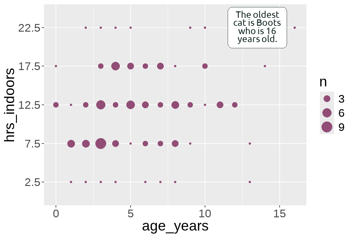

title <- "Do older cats spend more time indoors?"
perc_indoor <- round(100 * sum(cats_uk_reference$hrs_indoors == "22.5") / nrow(cats_uk_reference))
st <- glue("Around {perc_indoor}% of cats in the study spend on average 22.5 hours per day indoors! There is a slight trend for cats to spend more time indoors as they age.")
cap <- "Data: McDonald JL, Cole H. 2020 | Graphic: Nicola Rennie"

text_plot <- annotated_plot +
  labs(
    title = title,
    subtitle = st,
    caption = cap,
    x = "Age of cat (years)",
    y = "Average time spent indoors (hours per day)",
    size = "Number of cats"
  )
text_plot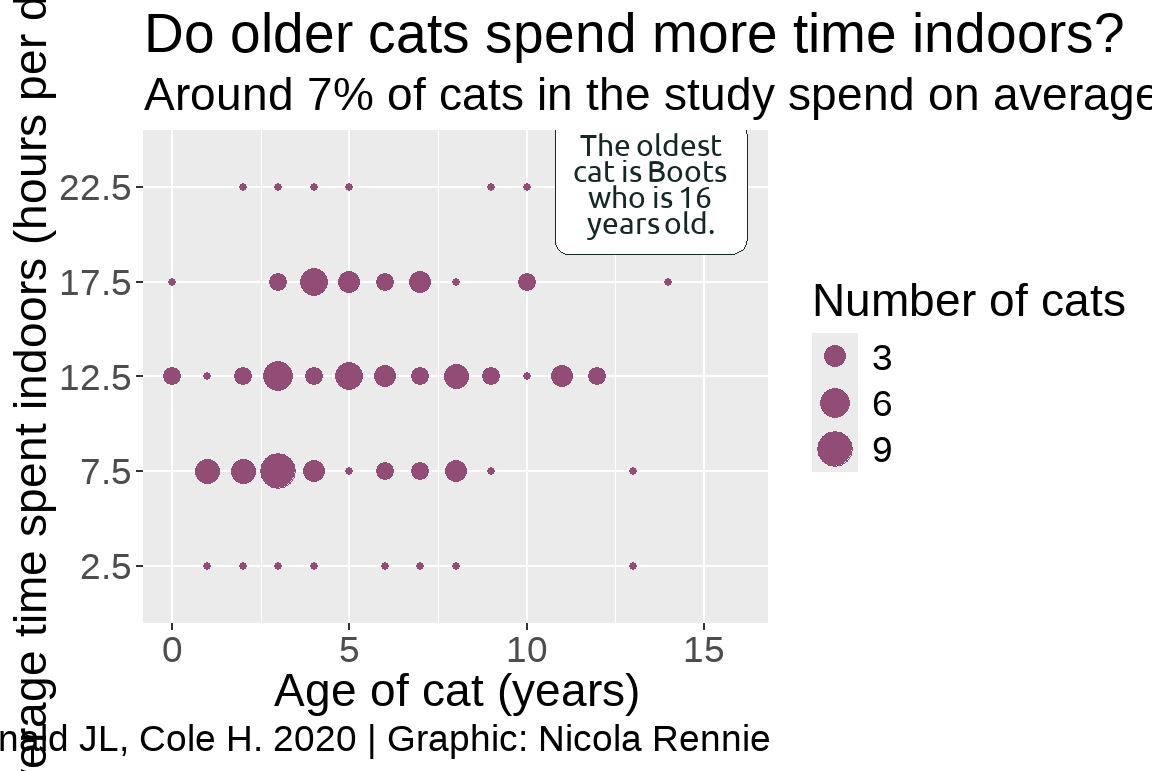

Themes

theme_plot1 <- text_plot +
  theme_minimal(
    base_family = body_font,
    base_size = 8
  )
theme_plot1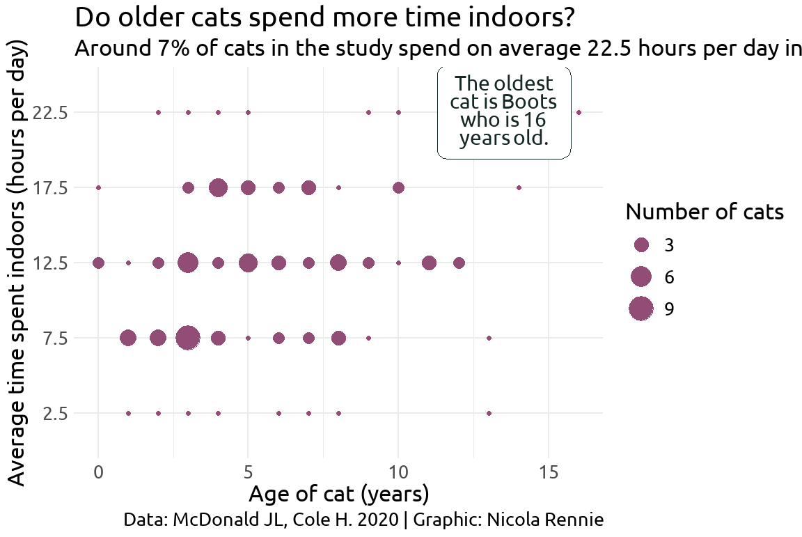

theme_plot2 <- theme_plot1 +
  theme(
    # legend styling
    legend.position = "inside",
    legend.position.inside = c(0.9, 0.25),
    legend.background = element_rect(fill = alpha(bg_col, 0.6), color = text_col),
    # text
    text = element_text(color = text_col),
    plot.title = element_text(family = title_font, face = "bold", size = rel(1.5)),
    plot.subtitle = element_textbox_simple(),
    plot.caption = element_textbox_simple(),
    plot.title.position = "plot",
    plot.caption.position = "plot",
    # background and grid
    panel.grid.minor = element_blank(),
    plot.background = element_rect(fill = bg_col, color = bg_col)
  )
theme_plot2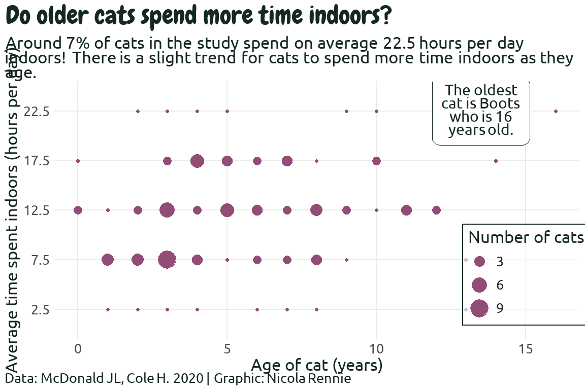

Saving

ggsave(
  theme_plot2,
  filename = "cats.png",
  width = 6,
  height = 4
)

If you’ve used ggview, then assign the plot to a variable e.g. p and then do:

save_ggplot(
  plot = p,
  file = "cats.png"
)